##############################
##         IMPORTS          ##
##############################
# Used to import and store the data
import pandas as pd
# Used for plotting
import matplotlib.pyplot as plt
# Needed to compute sums of lists
import numpy as np
#k-Nearest Neighbors
from sklearn.neighbors import KNeighborsClassifier
# Train-test split
from sklearn.model_selection import train_test_split
# Accuracy Score
from sklearn.metrics import accuracy_score
# Confusion Matrix
from sklearn.metrics import ConfusionMatrixDisplayPython Homework 3: Example Solutions
These are example solutions to the third Python homework, involving performing k-nearest neighbors classification on the titanic data set. Other correction solutions and implementations are possible.
##############################
 ##  IMPORT THE DATA SETS   ##
##############################
# Import the three data files
train = pd.read_csv("../DataSets/titanic_train.csv")
test = pd.read_csv("../DataSets/titanic_test.csv")
complete = pd.read_csv("../DataSets/titanic_test_complete.csv")
# Drop the Cabin column from each of the Dataframes as
# we will not use it later and it contains a lot of
# null values
train = train.drop(columns=["Cabin"])
test = test.drop(columns=["Cabin"])
complete = complete.drop(columns=["Cabin"])
# Drop the null values from each dataframe
train = train.dropna()
test = test.dropna()
complete = complete.dropna()######################################
## CONVERT CATEGORICAL TO NUMERICAL ##
#####################################
# Sex will likely be important (women and children first)
# Convert Sex from a categorical variables to a
# numeric variable for each of the three files./
train["Sex"] = pd.Categorical(train["Sex"])
train["Sex_Codes"] = train.Sex.cat.codes
test["Sex"] = pd.Categorical(test["Sex"])
test["Sex_Codes"] = test.Sex.cat.codes
complete["Sex"] = pd.Categorical(complete["Sex"])
complete["Sex_Codes"] = complete.Sex.cat.codes##############################
## CORRELATION MATRIX ##
##############################
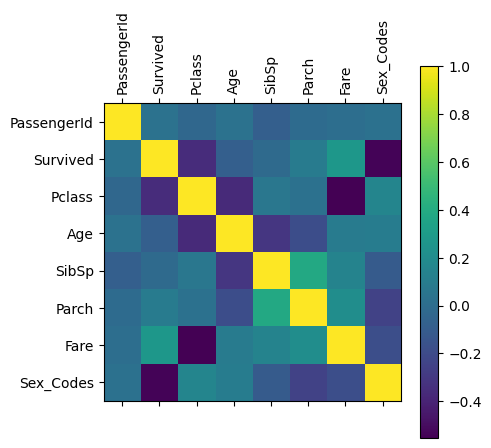
# Create a correlation matrix to determine which data is most
# correlated with the survived column
train_corr_matrix = train.corr(numeric_only=True)
# Display the correlation matrix with a colar bar
plt.matshow(train_corr_matrix)
plt.colorbar()
# Set the x and y tick marks to be the labels from the
# Dataframe
plt.xticks(range(len(train_corr_matrix)), train_corr_matrix,
rotation=90)
plt.yticks(range(len(train_corr_matrix)), train_corr_matrix)([<matplotlib.axis.YTick at 0x28656c8e0>,
<matplotlib.axis.YTick at 0x28656c160>,
<matplotlib.axis.YTick at 0x286532e50>,
<matplotlib.axis.YTick at 0x2865f5610>,
<matplotlib.axis.YTick at 0x2865eb100>,
<matplotlib.axis.YTick at 0x2865f5f10>,
<matplotlib.axis.YTick at 0x2865fea00>,
<matplotlib.axis.YTick at 0x2866024f0>],
[Text(0, 0, 'PassengerId'),
Text(0, 1, 'Survived'),
Text(0, 2, 'Pclass'),
Text(0, 3, 'Age'),
Text(0, 4, 'SibSp'),
Text(0, 5, 'Parch'),
Text(0, 6, 'Fare'),
Text(0, 7, 'Sex_Codes')])
###################################
## DEFINE TRAINING AND TEST SETS ##
###################################
# Let's take the three most correlated columns to survivors found above
# (Pclass, Fare, and Sex_Codes) as well as Age (women and children first)
# to define the X component. The training set comes from the train file
# and the test set comes from the test file.
X_train = train[['Pclass', 'Fare', 'Sex_Codes', 'Age']]
X_test = test[['Pclass','Fare','Sex_Codes', 'Age']]

# The y data is the survived column. The training set comes from the train
# file and the test set comes from the complete file.
y_train = train['Survived']
y_test = complete['Survived']
##############################
## INITIAL TRAINING ##
##############################
# Define the classifier
knn = KNeighborsClassifier(n_neighbors=3)
# Fit the classifier with the training data
knn.fit(X_train, y_train)
# Generate predictions for the test set
y_pred = knn.predict(X_test)
# Print the total number of survivors in the predicted set
print("Number of Surivors in Prediction:", np.sum(y_pred))
# Print the total number of survivors in the test set
print("Number of Survivors in Actual:", np.sum(y_test))
# Print the accuracy score between the predicted and test sets
print("Accuracy:", accuracy_score(y_test, y_pred)*100)Number of Surivors in Prediction: 131
Number of Survivors in Actual: 136
Accuracy: 48.94259818731118##############################
## HYPERPARAMETER TUNING ##
##############################
for k in range(1,20):
# Define the classifier
knn = KNeighborsClassifier(n_neighbors=k)
# Fit the classifier with the training data
knn.fit(X_train, y_train)
# Generate predictions for the test set
y_pred = knn.predict(X_test)
print("k:", k, "Accuracy:", accuracy_score(y_test, y_pred)*100)k: 1 Accuracy: 54.68277945619335
k: 2 Accuracy: 53.17220543806647
k: 3 Accuracy: 48.94259818731118
k: 4 Accuracy: 53.17220543806647
k: 5 Accuracy: 52.567975830815705
k: 6 Accuracy: 52.567975830815705
k: 7 Accuracy: 51.66163141993958
k: 8 Accuracy: 51.3595166163142
k: 9 Accuracy: 50.755287009063444
k: 10 Accuracy: 53.17220543806647
k: 11 Accuracy: 51.66163141993958
k: 12 Accuracy: 52.87009063444109
k: 13 Accuracy: 52.26586102719033
k: 14 Accuracy: 51.963746223564954
k: 15 Accuracy: 51.3595166163142
k: 16 Accuracy: 53.47432024169184
k: 17 Accuracy: 52.26586102719033
k: 18 Accuracy: 54.0785498489426
k: 19 Accuracy: 53.17220543806647##################################################
## PREDICTION WITH THE BEST NUMBER OF NEIGHBORS ##
##################################################
# Define the classifier
knn = KNeighborsClassifier(n_neighbors=16)
# Fit the classifier with the training data
knn.fit(X_train, y_train)
# Generate predictions for the test set
y_pred = knn.predict(X_test)
# Print the total number of survivors in the predicted set
print("Number of Surivors in Prediction:", np.sum(y_pred))
# Print the total number of survivors in the test set
print("Number of Survivors in Actual:", np.sum(y_test))
# Print the accuracy score between the predicted and test sets
print("Accuracy:", accuracy_score(y_test, y_pred)*100)Number of Surivors in Prediction: 116
Number of Survivors in Actual: 136
Accuracy: 53.47432024169184For the solutions to Questions 2 and 3, see the machine learning and classification notes.