Lecture Notes: Introduction to Excel (Excel Basics)
Microsoft Excel is a very powerful tool for visualizing and manipulating data. Unlike the other tools we will learn later in this course, Excel has a graphical user interface (GUI) that we can interact with. However, we will use a small amount of programming to perform some calculations and we will need to use computational thinking to break problems down into pieces which can be analyzed using Excel.
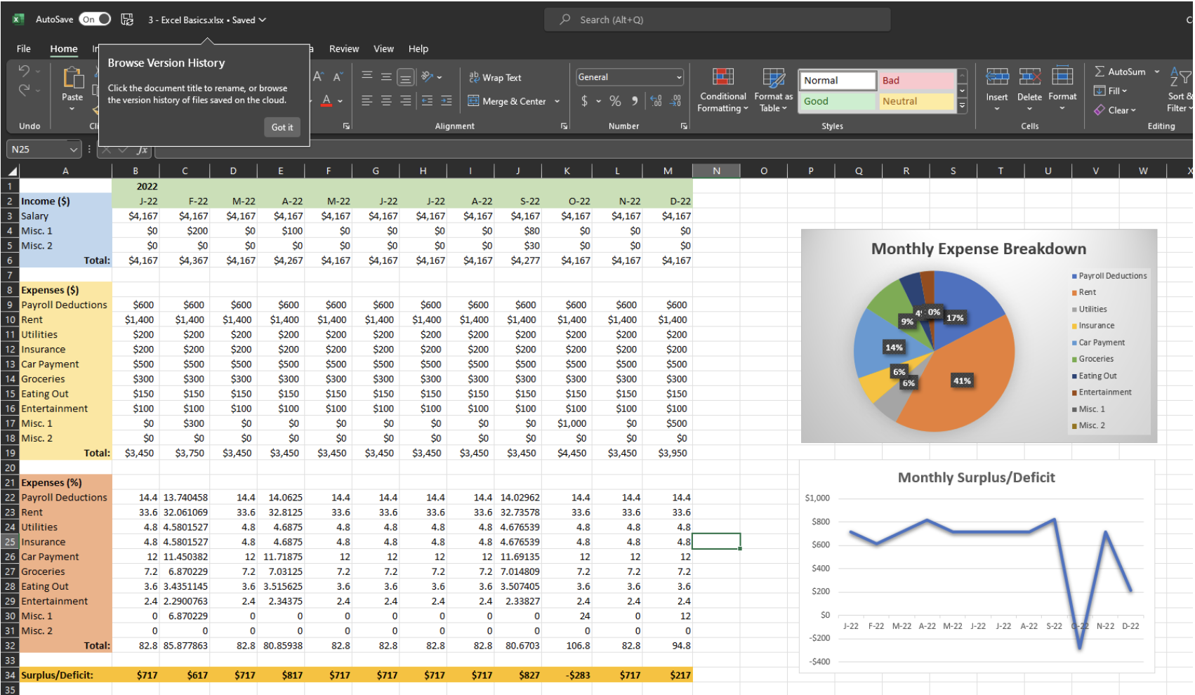
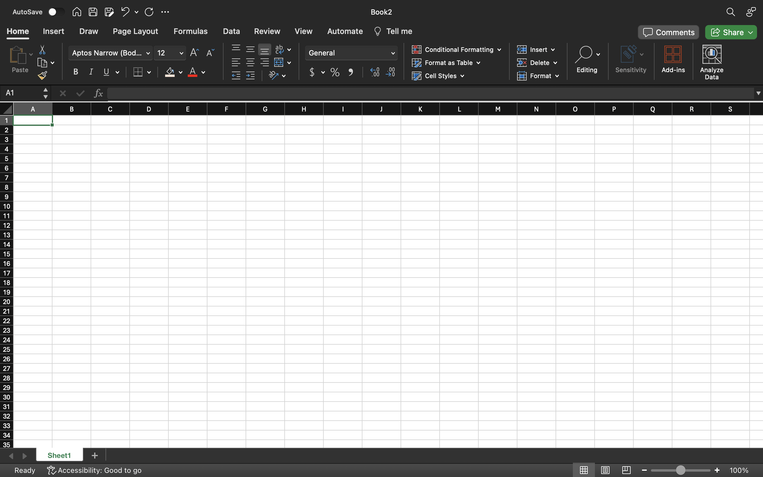
When you first open Excel after installing it, you will see a window that looks similar to the screenshot below. Note that my Excel is set to dark mode so the colors on your screen may be different depending on your computer settings. If you use other Microsoft Office products, such as Word or PowerPoint, then the top menu will look familar. If you do not use these product, no worries! We will learn the layout of the menu bar and the important options over the next coupled of weeks.
Below the menu bar is a grid that is organized using letters to denote the columns and numbers to denote the rows. Each grid block is called a cell and we will use these cells to input data and perform calculations. In today’s class we will input data into the cells ourselves by typing it in (and using the auto-fill feature!. In future classes, we will import our starting data from a different file.
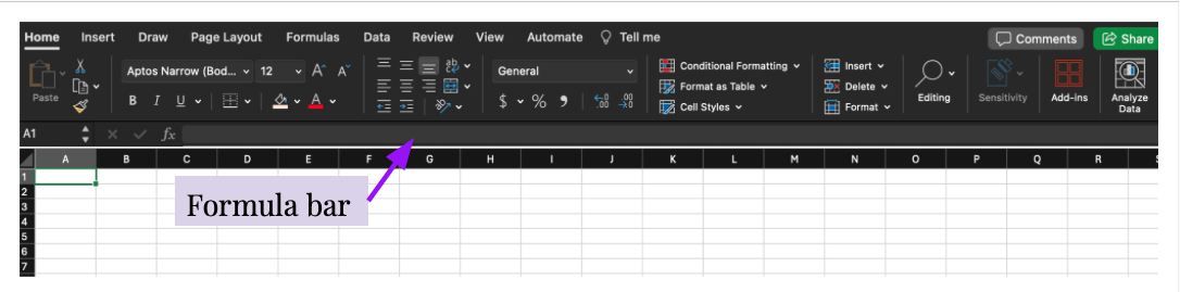
There are two ways to manually enter data into an Excel cell. First, you can click on a cell and just begin typing, what you type will appear in the cell. This is convenient if you are only typing something short. The second method, which is better if you need to type something longer into a cell, is to click the cell and then click the formula bar which is located below the menu bar and above the letters denoting the columns (shown in the figure below). You can then type into the formula bar and what you type will appear in the cell you clicked on first.
Creating a Credit Card Data Set
Autofill and Basic Formulas
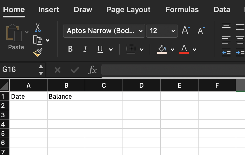
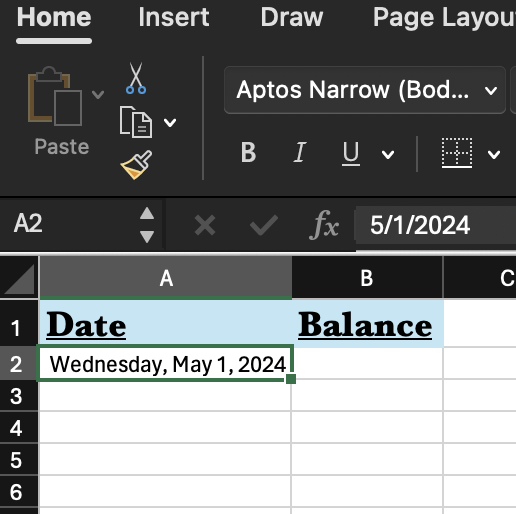
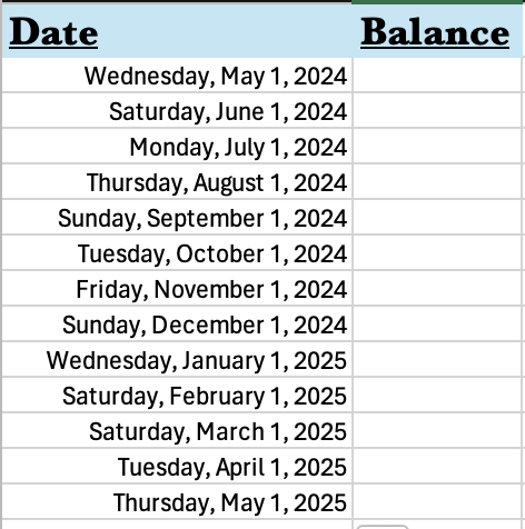
The goal of the project we will be completing today is to create a spreadsheet which will track our monthly income and expenses. We will start by creating a credit card tracker, which will calculate the balance on a credit card on the first of each month. To get started, type the phrase “Date” in cell A1 and the phrase “Balance” in the cell B1 using the method of your choice. Your Excel sheet should now look like this.
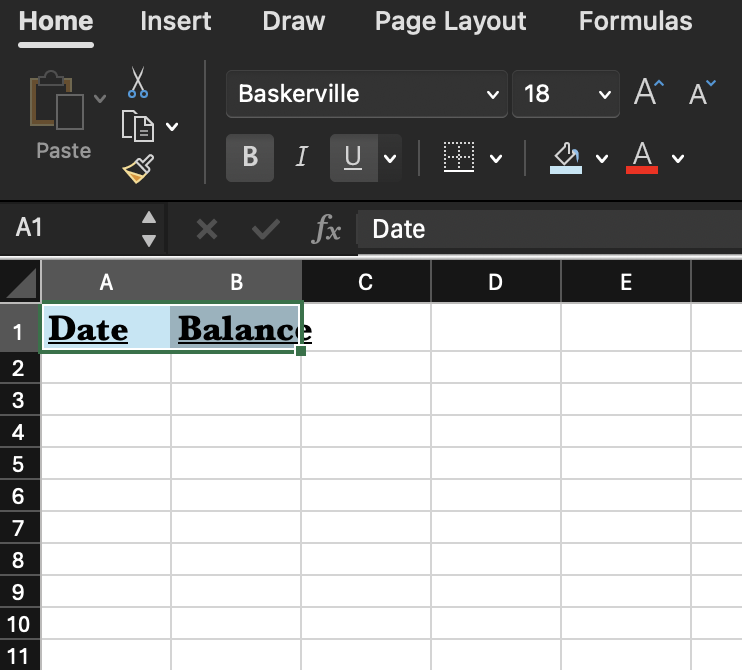
Next we can format the text in these cells. You can click and drag to select both of the code cells. You can then use the menu bar or keyboard shortcuts to format the text as bolded, italics, or underlined (the keyboard shortcuts are Control+B for bold, Control+I for italics, and Control+U for underline for a Windows or Linux computer and Command+B for bold, Command+I for italics, and Command+I for italics for Macs). You can also use the top menu bar to change the font type, size, color, and highlighter. Format these two header cells as you desire. An example is shown below.
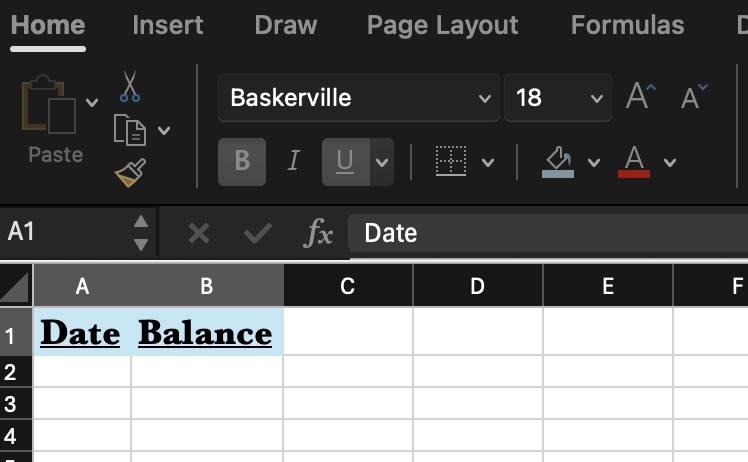
Note that in the above screenshot, I increased the font size of the text and now the cell is too small. You can resize a cell by clicking on the boundary between columns (or rows) and dragging it to the appropriate size. You can also double click on one of the boundaries to have it auto-size to the correct width or height. After resizing, my code cells look like this.
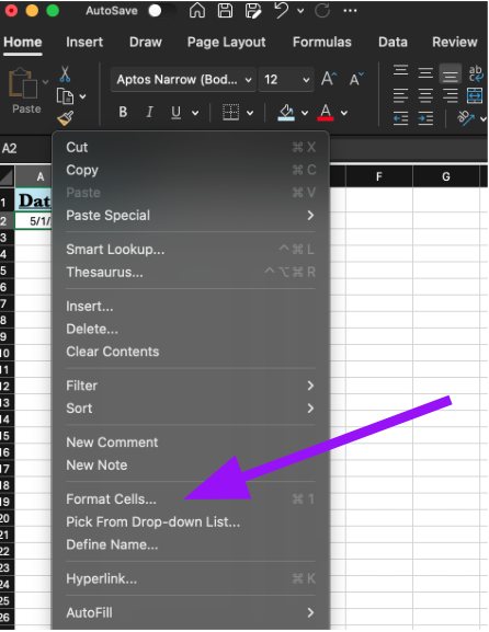
Under the dates column we want to enter a date corresponding to the first of the month (the example on the slides has the starting date as 9/1/22 but you are welcome to update it). Under the date you want to start with (needs to be the first of the month) in the form MM/DD/YYYY and then press the Enter/Return key. Now right-click on the cell and click “Format Cells” from the pop-up menu.
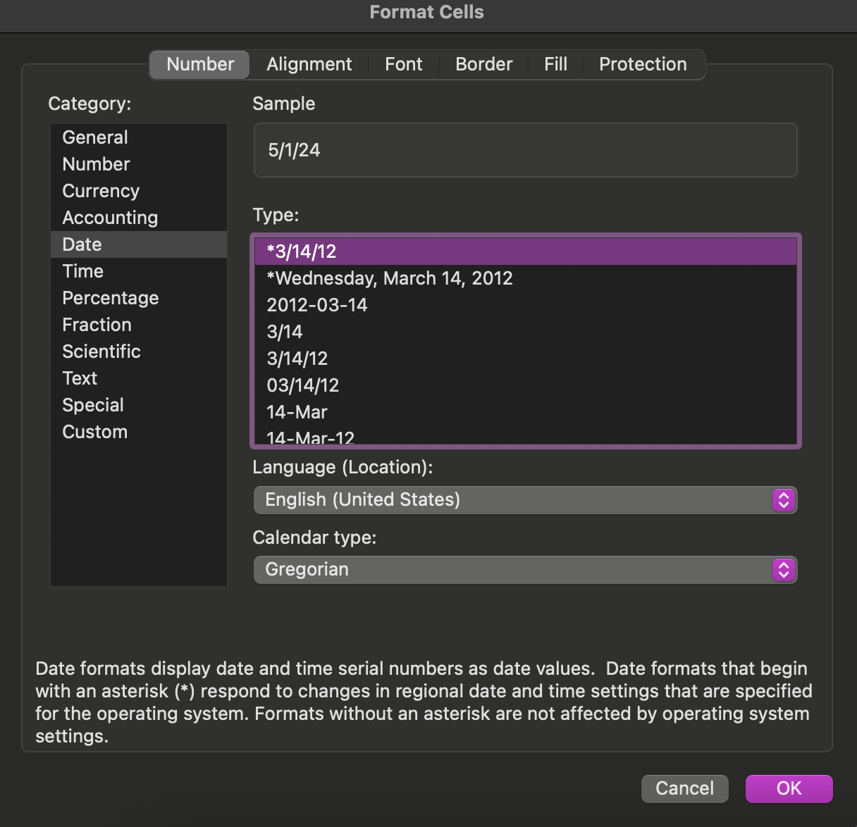
On the window that pops up you will see many options to format dates (this should be the default window which appears). Select a date format you like and then click “OK” at the bottom of the window. Your date should not be formatted in the style you selected.
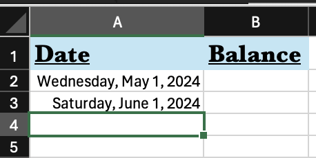
Now we want to fill the date column with the first day of each month. The nice thing about Excel is it will let us add a set number to a date and will convert that to mean jumping that number of days in the future. So, to generate the next month, go to the next cell (this should be A3) and type =A2+31 (note that I used 31 here because May has 31 days, you can adjust this as needed for your starting month). As an alternative, you can click on cell A3, type =, then click on cell A2, and then type +31. This method may seem like more steps but it is more convienint in most cases because it means you do not need to know the exact letter and number combination of the cell you want to use. After doing this, you should have something similar to the below picture, where the new date will autoformat to match the style you chose for the first date.
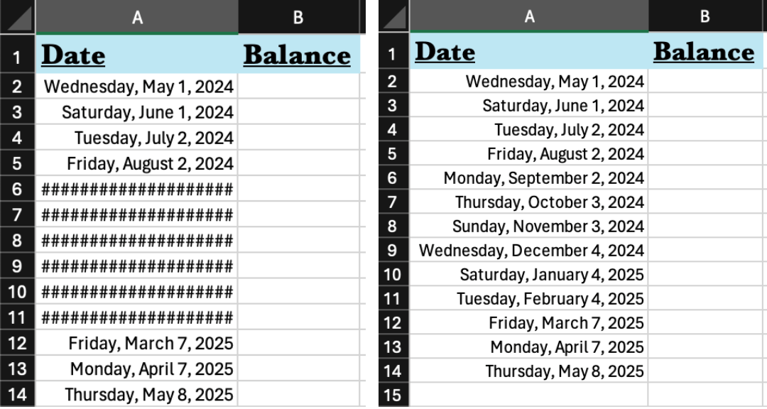
We have now established a pattern in the column (i.e. the next cell should be the previous cell +31 (or the number you chose)). If you click on cell A3 there should be a small square box in the bottom right corner. Click that box and drag it down to cell A14 to create more dates. This is called auto-filling, Excel is actually pretty good at recognizing patterns and recreating them. You should end up with something like this. Note that if your column is too narrow, when you release the auto-fill you may get a bunch of cells that are filled with number signs (##############). Simply widen the column and the dates should appear. You should end up with something similar to the below image.
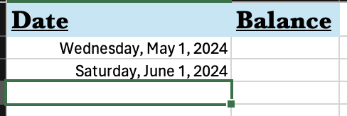
However, there is a problem which what we currently have: months are not the same length so our dates start to get off-set from the 1st. Let’s delete what we have done by highlighting cells A3-A14 and hitting the delete key. We need to find a way to increment only the month but not the day. To accomplish this, click on cell A3 and then type =DATE(YEAR(A2),MONTH(A2)+1,DAY(A2)). This is a function, and our first example of programming in Excel. The DATE function takes three arguments, the year, month, and the day. Arguments are the parameters a function needs to perform its operation. In this case, if we pass it a year, a month, and a day it will format the result as a date. We will take the year from cell A2 by using the YEAR function and passing it the cell A2 as an argument. For the month we take the month from cell A2 with the MONTH function but add 1 to it to increment the month. Finally, we take the day from cell A2 using the DAY function. You should now have something that looks like this.
We can now click on the small square at the bottom right of cell A3 and drag it down to cell A14 to autofill just the first of the next months. We now have a year of dates for the first of every month without having to type them all in!
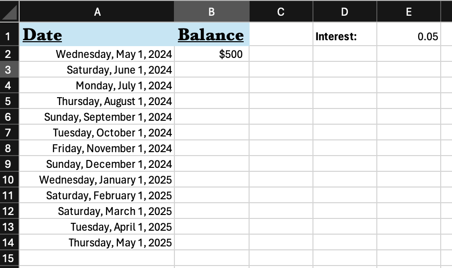
Now in the balance column we want to calculate the balance on a credit card that accumulates interest monthly but receives no payments. In cell D1 create a header entitled Interest and then in cell E1 type =5%. (This is a very small interest rate for a credit card …) Note that after you hit Enter/Return after typing this the cell will reformat to 0.05. Finally, add a balance of $500 to cell B2 (type $500). You should now have a spreadsheet which looks like the below screenshot. Fill free to change the fonts or colors if you desire.
We now want to create a formula which will calculate the credit card balance including the interest for each of the dates we have in column A. The formula to calculate the interest for a credit card is:
\[P = P_0(1+i),\]
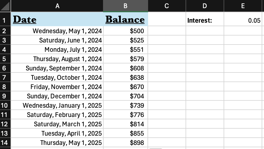
where \(P_0\) is the prior month’s balance, i is the interest rate (0.05 for 5% interest) and P is the amount which will be on the credit card after interest is applied. To start this calculation, we can type =B2*(1+E1) in cell B3 to calculate the balance on the credit card after interest is applied. After this, click the small box at the bottom right corner of B3 and drag it down to B14 to auto-fill. After you do this you should have the following spreadsheet.
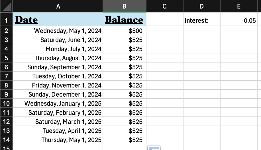
If you look closely, the interest was applied correctly on the first month but was never applied again. If you click on cell B14 and look at the interest bar, you will see that Excel attempted to continue our pattern by incrementing the row number for the B column (which we want) but also by incrementing the row number of the E column (which we do not want). We want E1 to stay fixed because that is where we added the interest. Luckily the solution to this is quite easy: just change the formula in cell A3 to =A2*(1+E$1) and redo the auto-fill. The $ tells Excel not to increment the row number (it locks the row number). You can also add a $ in front of a column letter to lock that if needed as well. With this correction your spreadsheet should now be correct.
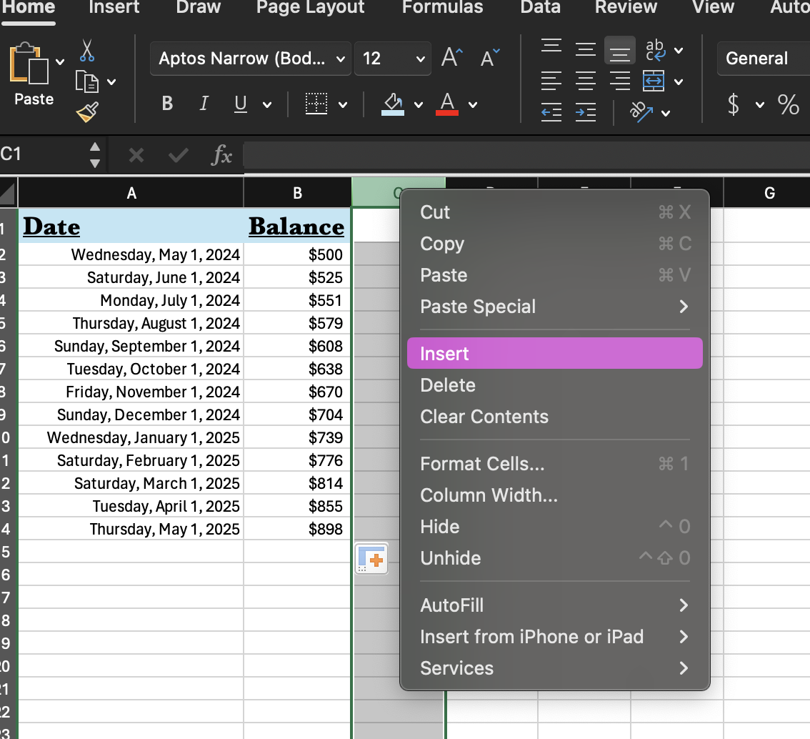
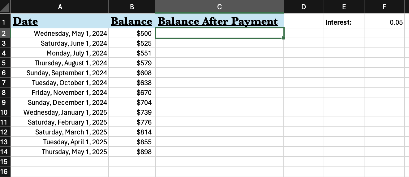
Turns out, if you do not make credit card payments the interest adds up quickly! So let’s add to the spreadsheet a column that will show the balance if we make a payment each month. First, we want to add a new column beside the Balance column. Right-click on the C column and click insert. This will create a new column that we can use to calculate the balance after payments are made. Name this column Balance After Payment and format and resize as needed. Note that after you insert the column, the formulas in column B will automatically update.
Create a header called Payment in cell E2 and define a minimum payment of $25 in cell F2.
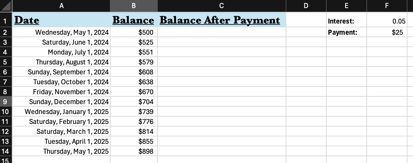
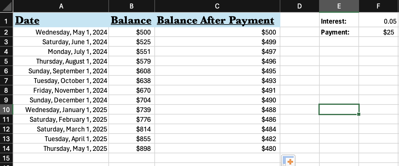
Add the initial balance of $500 to cell C2. The new equation for interest while making a monthly payment is:
\[P = (P_0-p)(1+i),\]
where p is the payment being made each month. To convert this equation to code, type =(C2-F$2)(1+F$1) in cell C3 and then auto-fill all the way down to C14. Note that the balance owed does decrease, but it decreases very slowly.
Creating Graphs in Excel
Now that we have created two data sets (credit card balance without payment and credit card balance with payment) let’s create a graph that shows the balance as a function of the month. Start by highlighting all of the data (cells A1 through C14). Now click “Insert”, then click the line graph symbol, and finally click on the “Line with Markers” graph. When you click on this a graph will appear. If it covers the data you can change its position by clicking it and dragging it to a new location.
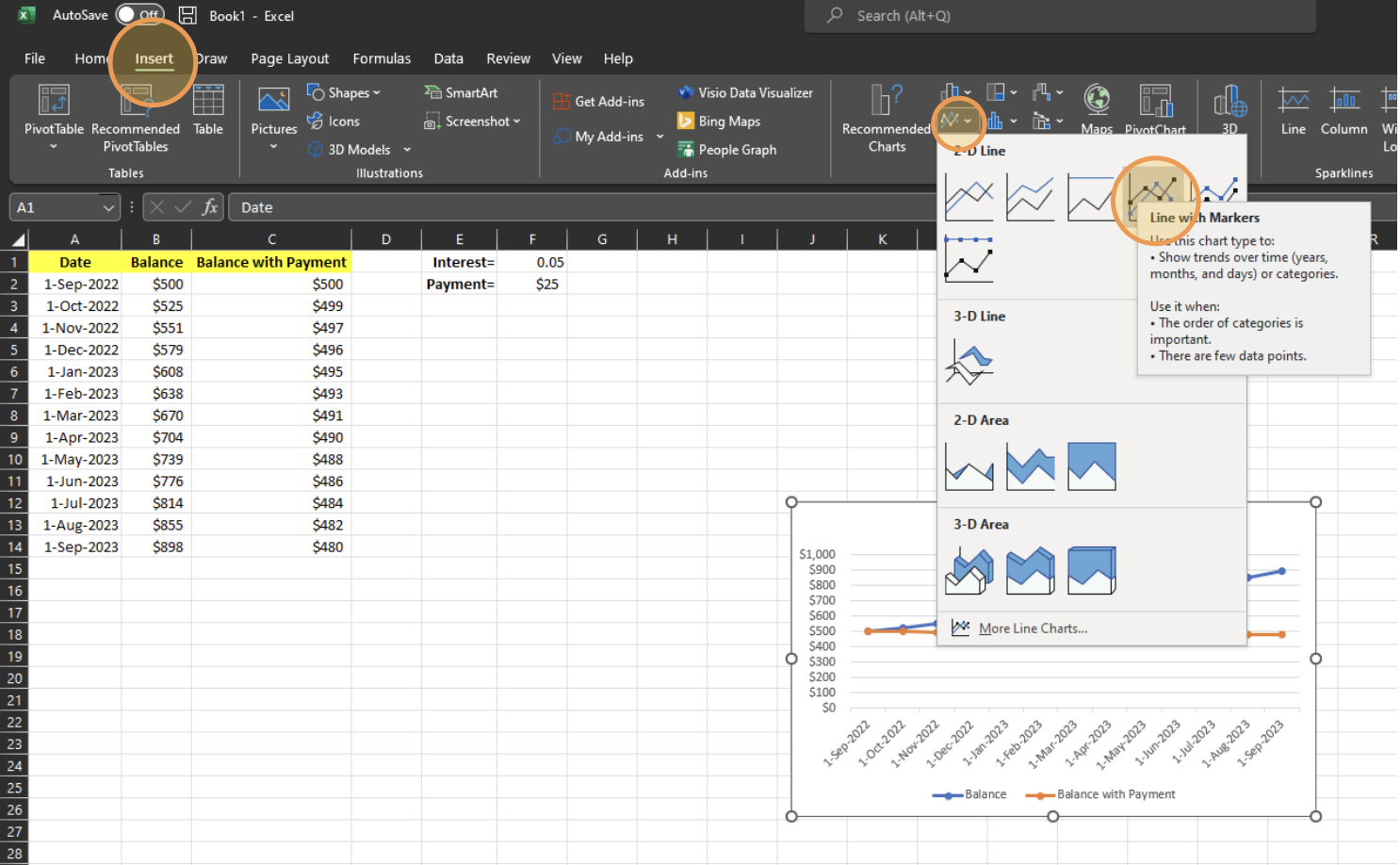
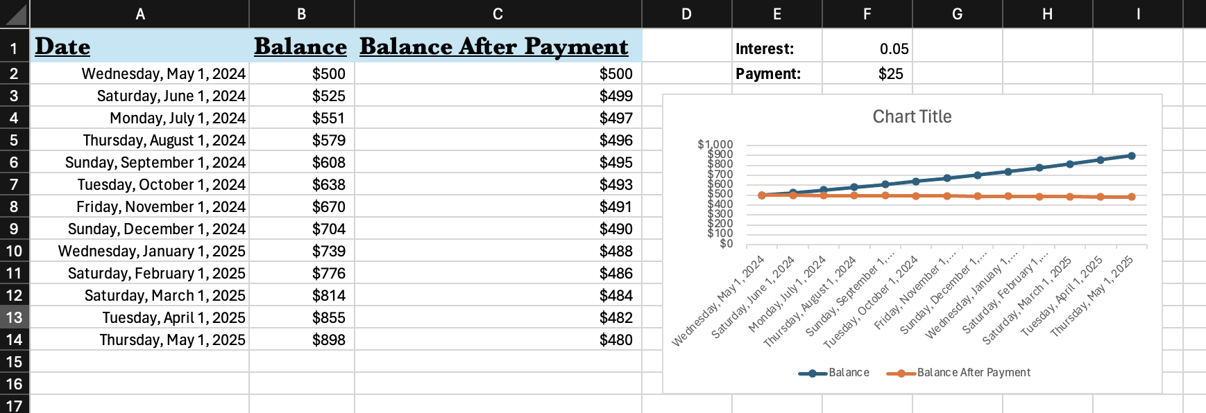
A small graph of our data has now been created. Note that Excel automatically created the data using column A for the x-axis and columns B and C as two different data sets. The two data sets were given different colors and a legend was automatically collected using the headers in row 1. You can resize the graph as needed by clicking and dragging any of the corners.
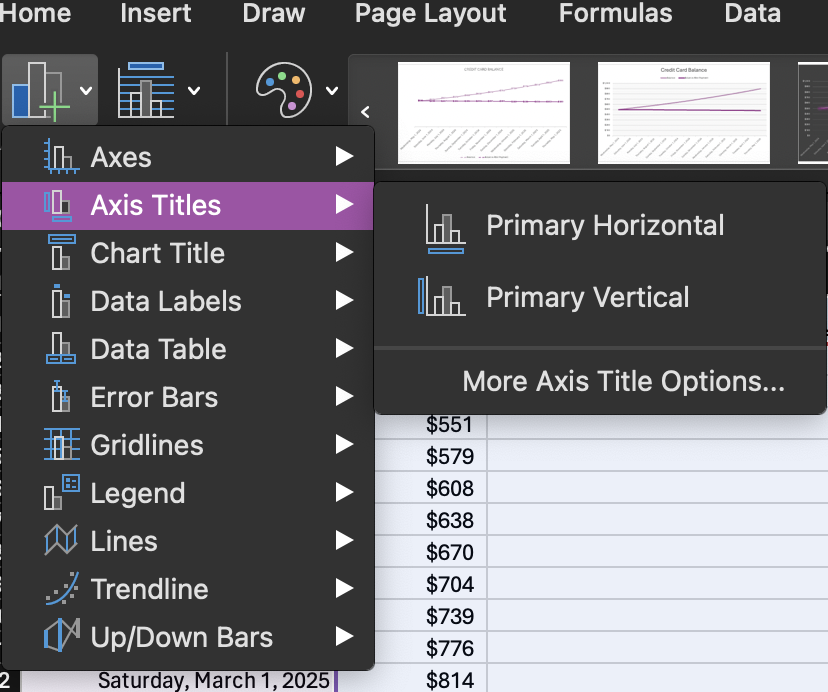
You can click the phrase Chart Title and edit it to reflect what is being graphed. The “Char Design” Tab in the menu bar has many options for formatting the graph and adding new elements to it. You can play around with some of the pre-set designs on this menu to find one you like. You can also change the colors using the “Change Colors” menu. A good graph needs both an x and y axes label. You can add these from the “Chart Design” menu, using the “Add Chart Element” drop-down menu, then “Axis Titles”; you want to add both horizontal and vertical axis titles. You can change the text of the placeholders by clicking on them.
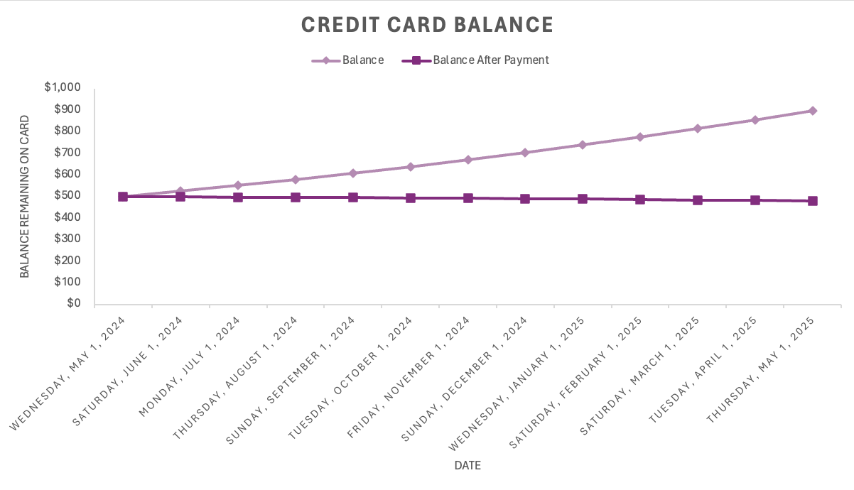
Eventually, you will create a graph that you are happy with!
Once you have your graph, at the bottom of the Excel window, double click on the sheet name “Sheet 1” and rename it to “Credit Card”. Click the “+” icon to create a new sheet. This will be another blank spreadsheet. Name this sheet “Budget”. Now you will have a chance to practice the skills you have learned by completing a simple project where you will use Excel to calculate a budget and create graphs. The final spreadsheet will look like this. The project guidelines are available here.