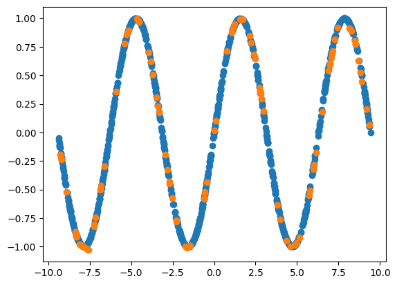
While regular neural networks perform well at interpolation, they tend to perform poorly when asked to extrapolate (this is a fact that is true of most machine learning algorithms)
Many extrapolation cases with machine learning use recurrent neural networks
While traditional neural networks are feedforward (data only passes from input layer to output layer) recurrent neural networks have a memory that feeds information backwards
rnn
Note that the input data for an RNN for both training and testing needs to be three dimensional.
SimpleRNN has the same arguments as Dense where the number is the number of neurons and we can set the activation function.
Note that you still need at least one Dense layer at the end of the network to “post-process” the results
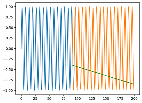
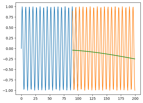
X_train = np.arange(0,100,0.5) y_train = np.sin(X_train)X_test = np.arange(90,200,0.5) y_test = np.sin(X_test)# Preprocess the data for the RNNX_train = X_train.reshape(-1, 1, 1) # Reshape the input data for RNN# Create the RNN modelmodel = tf.keras.Sequential([ tf.keras.layers.SimpleRNN(32, activation='relu', input_shape=(1, 1)), tf.keras.layers.Dense(1)])# Compile the modelmodel.compile(optimizer='adam', loss='mean_squared_error')# Train the modelmodel.fit(X_train, y_train, epochs=100, verbose=0)X_test = X_test.reshape(-1, 1, 1)y_pred = model.predict(X_test)print(mse(y_test.flatten(), y_pred))plt.plot(X_train.flatten(), y_train)plt.plot(X_test.flatten(), y_test)plt.plot(X_test.flatten(), y_pred, color='green')
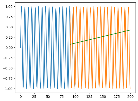
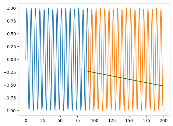
Some applications of RNNs have shown that in addition to using Dense layers to post-process the results of RNN layers, Dense layers can also be used to pre-process the results before they reach the RNN layers
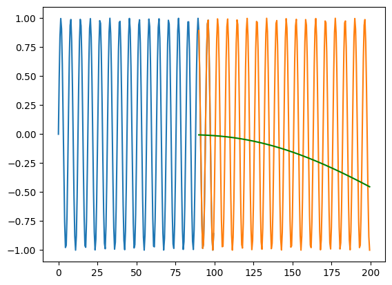
X_train = np.arange(0,100,0.5) y_train = np.sin(X_train)X_test = np.arange(90,200,0.5) y_test = np.sin(X_test)# Preprocess the data for the RNNX_train = X_train.reshape(-1, 1, 1) # Reshape the input data for RNN# Create the RNN modelmodel = tf.keras.Sequential([ tf.keras.layers.Dense(32, activation='relu', input_shape=(1, 1)), tf.keras.layers.SimpleRNN(32, activation='relu', return_sequences=True), tf.keras.layers.SimpleRNN(32, activation='relu',return_sequences=True), tf.keras.layers.Dense(1)])# Compile the modelmodel.compile(optimizer='adam', loss='mean_squared_error')# Train the modelmodel.fit(X_train, y_train, epochs=100, verbose=0)X_test = X_test.reshape(-1, 1, 1)y_pred = model.predict(X_test)print(mse(y_test, y_pred.flatten()))plt.plot(X_train.flatten(), y_train)plt.plot(X_test.flatten(), y_test)plt.plot(X_test.flatten(), y_pred.flatten(), color='green')