##############################
##          IMPORTS         ##
##############################
import numpy as np
import seaborn as sns
import matplotlib.pyplot as plt


## SKLEARN = SCIKIT-LEARN LIBRARY
from sklearn import datasets
from sklearn.linear_model import LinearRegression
from sklearn.model_selection import train_test_split
from sklearn.metrics import r2_score, mean_squared_errorLinear Regression and the Machine Learning Workflow
CSC/DSC 340 Week 2 Slides
August 28 - September 1, 2023
Plans for the Week
Monday
- Lecture: “Linear Regression and the Machine Learning Workflow”
- Week 1 In-Class Assignment and Week 2 Pre-Class Due BEFORE MIDNIGHT
- Suggested Reading: Hands-On Chapter 2 and Chapter 4 (only about linear regression)
- Office hours: 1pm to 3pm
Wednesday
- Finish “Linear Regression and the Machine Learning Workflow”
- Start In-Class Assignment: Revisting Nuclear Binding Energies with Linear Regression
- Week 1 Post-Class Due
- Suggested Reading: Hands-On Chapter 2 and Chapter 4 (only about linear regression)
- Office hours: 4pm tp 6pm
Thursday
- Office hours: 11am to 1pm
Friday
- Finish In-Class Assignment: Revisting Nuclear Binding Energies with Linear Regression
- Suggested Reading: Hands-On Chapter 2 and Chapter 4 (only about linear regression)
Next Week
- No class on Monday (Labor Day)
- In-Class Week 2, Pre-Class Week 3, and Post-Class Week 3 all due Wednesday before class
Part 1: Linear Regression
# Create a linear data set with a slope of 4 and an intercept of -3
X = np.arange(-5,5)
y = 4*X-3

plt.plot(X,y, color='blue',linewidth=3)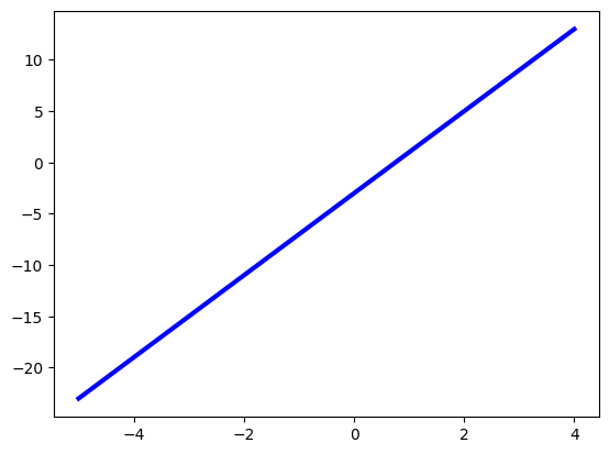
Goal: Find a line which fits the data set and can be used to predict new points from the data set
Linear Regression
\[\hat{y} = X\theta\]
- \(\hat{y}\): Machine learning predictions (a vector)
- \(X\): x-data, input data, features (vector or matrix)
- \(\theta\): parameters or weights of the algorithm (vector)
- y: known output data (targets or labels)
Goal: Find \(\theta\) such that \(\hat{y} \approx y\)
Linear Regression Loss Function
Mean-Squared Error Function:
\[J_{MSE}(\theta) = \frac{1}{N}\sum_{i=1}^N (\hat{y}_i - y_i)^2\]
Re-write using linear regression:
\[J_{MSE}(\theta) = \frac{1}{N}\sum_{i=1}^N (X_i\theta - y_i)^2\]
Convert to matrix-vector notation: \[ J_{MSE}(\theta) = \frac{1}{N}[X\theta - y]^T[X\theta - y]\]
Find Optimized Weights
Loss Function:
\[ J(\theta) = \frac{1}{N}[X\theta - y]^T[X\theta - y]\]
Optimize with respect to \(\theta\) (minimization problem):
\[\frac{\partial J(\theta)}{\partial \theta} = 0 \]
Apply to the loss function:
\[ \frac{\partial}{\partial \theta} \{\frac{1}{N}[X\theta - y]^T[X\theta-y]\} = 0\]
Take the derivative:
\[X^T[X\theta - y] = 0\]
Solve for \(\theta\):
\[ \theta = (X^TX)^{-1}X^Ty\]
Then to find prediction for new y-data points:
\[\hat{y} = X_{new}\theta = X_{new}(X^TX)^{-1}X^Ty,\]
where X, y are known as the training data (the data used to find the optimized parameters)
A closed-form solution!
Implementing Linear Regression with Sklearn
# Create a linear regression instance using sklearn
linear_regression = LinearRegression()

# If the x-data in 1D, reshape as follows
X = X.reshape(-1,1)

# Fit the linear regression algoritm using the previously generated data
linear_regression.fit(X,y)LinearRegression()In a Jupyter environment, please rerun this cell to show the HTML representation or trust the notebook.
On GitHub, the HTML representation is unable to render, please try loading this page with nbviewer.org.
LinearRegression()
# Create new data from the same line in order to test its performance
X_test = np.arange(-10,10,0.1)
y_test = 4*X_test-3

X_test = X_test.reshape(-1,1)

y_pred = linear_regression.predict(X_test)
# Graphically check to see if the true and predicted data are similar
plt.plot(X_test,y_test,color='blue',linewidth=3,label="True")
plt.plot(X_test, y_pred, color='red', linewidth=3,linestyle=':', label="Predicted")
plt.legend()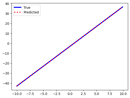
# Check accuracy using traditional error scores (MSE, RMSE, r2-score, percent error, etc.)
print("MEAN SQUARED ERROR:", mean_squared_error(y_test, y_pred))
print("ROOT MEAN SQUARED ERROR:", np.sqrt(mean_squared_error(y_test, y_pred)))
MEAN SQUARED ERROR: 1.7369681753028576e-28
ROOT MEAN SQUARED ERROR: 1.3179408846009966e-14# Check the optimized weights and the slope that are fit by the linear regression algorithm
# The slope should be 4 and the intercept -3 (set when we created the data)
print("LINEAR REGRESSION SLOPE:", linear_regression.coef_)
print("LINEAR REGRESSION INTERCEPT:", linear_regression.intercept_)LINEAR REGRESSION SLOPE: [4.]
LINEAR REGRESSION INTERCEPT: -3.000000000000001Why start with linear regression?
- Simple machine learning model which has many of the feature of more complicated models
- A loss function
- Weights/parameters to be optimized
- A “training” process
- Closed-form for optimized weights means same results for the same data
- Many data sets follow a linear-ish pattern
- Linear regression can be modified to be more powerful with a design matrix (In-Class Assignment) or with regularization (next week)
Part 2: The Machine Learning Workflow with Linear Regression
The Machine Learning Workflow
- General Steps of any machine learning analysis:
- Import the data set, perform an initial analysis
- Split the data into a training set and a test set
- Train the machine learning algorithm with the training set
- Test the performance of the trained model with the test set using numerical metrics and visual analysis
- (Optional) Improve the performance of the algorithm by either reformatting the data OR changing the parameters of the machine learning algorithm
- Hands-On Machine Learning Chapter 2 has a detailed walkthrough
- Helpful Checklist: Appendix B
1. Import the data set, perform an initial analysis
- Importing the data set from a file, Python library, or website
- Determine what the data set contains
- Determine if any of the data needs to be modified or removed (missing values, non-numeric values, etc.) (Post-Class 2, Pre-Class 4)
- Perform initial analysis: Print the data, graph the data, modify the data if needed
The data set we will be analyzing is called the “Diabetes Data Set” and it contains data from 442 people. The goal of the data set is to predict a machine learning model that can tell how far diabetes has progressed in the patient given various health information.
# The data set is avaliable through Scikit-Learn
diabetes_data = datasets.load_diabetes()
diabetes_data
{'data': array([[ 0.03807591, 0.05068012, 0.06169621, ..., -0.00259226,
0.01990749, -0.01764613],
[-0.00188202, -0.04464164, -0.05147406, ..., -0.03949338,
-0.06833155, -0.09220405],
[ 0.08529891, 0.05068012, 0.04445121, ..., -0.00259226,
0.00286131, -0.02593034],
...,
[ 0.04170844, 0.05068012, -0.01590626, ..., -0.01107952,
-0.04688253, 0.01549073],
[-0.04547248, -0.04464164, 0.03906215, ..., 0.02655962,
0.04452873, -0.02593034],
[-0.04547248, -0.04464164, -0.0730303 , ..., -0.03949338,
-0.00422151, 0.00306441]]),
'target': array([151., 75., 141., 206., 135., 97., 138., 63., 110., 310., 101.,
69., 179., 185., 118., 171., 166., 144., 97., 168., 68., 49.,
68., 245., 184., 202., 137., 85., 131., 283., 129., 59., 341.,
87., 65., 102., 265., 276., 252., 90., 100., 55., 61., 92.,
259., 53., 190., 142., 75., 142., 155., 225., 59., 104., 182.,
128., 52., 37., 170., 170., 61., 144., 52., 128., 71., 163.,
150., 97., 160., 178., 48., 270., 202., 111., 85., 42., 170.,
200., 252., 113., 143., 51., 52., 210., 65., 141., 55., 134.,
42., 111., 98., 164., 48., 96., 90., 162., 150., 279., 92.,
83., 128., 102., 302., 198., 95., 53., 134., 144., 232., 81.,
104., 59., 246., 297., 258., 229., 275., 281., 179., 200., 200.,
173., 180., 84., 121., 161., 99., 109., 115., 268., 274., 158.,
107., 83., 103., 272., 85., 280., 336., 281., 118., 317., 235.,
60., 174., 259., 178., 128., 96., 126., 288., 88., 292., 71.,
197., 186., 25., 84., 96., 195., 53., 217., 172., 131., 214.,
59., 70., 220., 268., 152., 47., 74., 295., 101., 151., 127.,
237., 225., 81., 151., 107., 64., 138., 185., 265., 101., 137.,
143., 141., 79., 292., 178., 91., 116., 86., 122., 72., 129.,
142., 90., 158., 39., 196., 222., 277., 99., 196., 202., 155.,
77., 191., 70., 73., 49., 65., 263., 248., 296., 214., 185.,
78., 93., 252., 150., 77., 208., 77., 108., 160., 53., 220.,
154., 259., 90., 246., 124., 67., 72., 257., 262., 275., 177.,
71., 47., 187., 125., 78., 51., 258., 215., 303., 243., 91.,
150., 310., 153., 346., 63., 89., 50., 39., 103., 308., 116.,
145., 74., 45., 115., 264., 87., 202., 127., 182., 241., 66.,
94., 283., 64., 102., 200., 265., 94., 230., 181., 156., 233.,
60., 219., 80., 68., 332., 248., 84., 200., 55., 85., 89.,
31., 129., 83., 275., 65., 198., 236., 253., 124., 44., 172.,
114., 142., 109., 180., 144., 163., 147., 97., 220., 190., 109.,
191., 122., 230., 242., 248., 249., 192., 131., 237., 78., 135.,
244., 199., 270., 164., 72., 96., 306., 91., 214., 95., 216.,
263., 178., 113., 200., 139., 139., 88., 148., 88., 243., 71.,
77., 109., 272., 60., 54., 221., 90., 311., 281., 182., 321.,
58., 262., 206., 233., 242., 123., 167., 63., 197., 71., 168.,
140., 217., 121., 235., 245., 40., 52., 104., 132., 88., 69.,
219., 72., 201., 110., 51., 277., 63., 118., 69., 273., 258.,
43., 198., 242., 232., 175., 93., 168., 275., 293., 281., 72.,
140., 189., 181., 209., 136., 261., 113., 131., 174., 257., 55.,
84., 42., 146., 212., 233., 91., 111., 152., 120., 67., 310.,
94., 183., 66., 173., 72., 49., 64., 48., 178., 104., 132.,
220., 57.]),
'frame': None,
'DESCR': '.. _diabetes_dataset:\n\nDiabetes dataset\n----------------\n\nTen baseline variables, age, sex, body mass index, average blood\npressure, and six blood serum measurements were obtained for each of n =\n442 diabetes patients, as well as the response of interest, a\nquantitative measure of disease progression one year after baseline.\n\n**Data Set Characteristics:**\n\n :Number of Instances: 442\n\n :Number of Attributes: First 10 columns are numeric predictive values\n\n :Target: Column 11 is a quantitative measure of disease progression one year after baseline\n\n :Attribute Information:\n - age age in years\n - sex\n - bmi body mass index\n - bp average blood pressure\n - s1 tc, total serum cholesterol\n - s2 ldl, low-density lipoproteins\n - s3 hdl, high-density lipoproteins\n - s4 tch, total cholesterol / HDL\n - s5 ltg, possibly log of serum triglycerides level\n - s6 glu, blood sugar level\n\nNote: Each of these 10 feature variables have been mean centered and scaled by the standard deviation times the square root of `n_samples` (i.e. the sum of squares of each column totals 1).\n\nSource URL:\nhttps://www4.stat.ncsu.edu/~boos/var.select/diabetes.html\n\nFor more information see:\nBradley Efron, Trevor Hastie, Iain Johnstone and Robert Tibshirani (2004) "Least Angle Regression," Annals of Statistics (with discussion), 407-499.\n(https://web.stanford.edu/~hastie/Papers/LARS/LeastAngle_2002.pdf)\n',
'feature_names': ['age',
'sex',
'bmi',
'bp',
's1',
's2',
's3',
's4',
's5',
's6'],
'data_filename': 'diabetes_data_raw.csv.gz',
'target_filename': 'diabetes_target.csv.gz',
'data_module': 'sklearn.datasets.data'}# Features: x-data set
# Data on each of the patients in the study
# How many features and data points?
print(diabetes_data.data.shape)
# What are the features?
print(diabetes_data.feature_names)(442, 10)
['age', 'sex', 'bmi', 'bp', 's1', 's2', 's3', 's4', 's5', 's6']Diabetes Dataset Feature Explanations
Note that all features data is mean-centered and scaled so the values do not reflect the actual measurements
| Feature Name | Explanation |
|---|---|
| age | Age of patient in years |
| sex | Biological sex of patient (male (0) or female (1) |
| bmi | Body mass index |
| bp | Blood pressure |
| s1 | Total serum cholestrol |
| s2 | Low-density lipoproteins |
| s3 | High-density lipoproteins |
| s4 | Total cholestrol |
| s5 | Log of serum triclyceride levels |
| s6 | Blood sugar |
# Targets: y-data set
# A quantitative measure of how far the disease has progressed
print(diabetes_data.target)
print("------------------------------------")
print(np.min(diabetes_data.target), np.max(diabetes_data.target))
[151. 75. 141. 206. 135. 97. 138. 63. 110. 310. 101. 69. 179. 185.
118. 171. 166. 144. 97. 168. 68. 49. 68. 245. 184. 202. 137. 85.
131. 283. 129. 59. 341. 87. 65. 102. 265. 276. 252. 90. 100. 55.
61. 92. 259. 53. 190. 142. 75. 142. 155. 225. 59. 104. 182. 128.
52. 37. 170. 170. 61. 144. 52. 128. 71. 163. 150. 97. 160. 178.
48. 270. 202. 111. 85. 42. 170. 200. 252. 113. 143. 51. 52. 210.
65. 141. 55. 134. 42. 111. 98. 164. 48. 96. 90. 162. 150. 279.
92. 83. 128. 102. 302. 198. 95. 53. 134. 144. 232. 81. 104. 59.
246. 297. 258. 229. 275. 281. 179. 200. 200. 173. 180. 84. 121. 161.
99. 109. 115. 268. 274. 158. 107. 83. 103. 272. 85. 280. 336. 281.
118. 317. 235. 60. 174. 259. 178. 128. 96. 126. 288. 88. 292. 71.
197. 186. 25. 84. 96. 195. 53. 217. 172. 131. 214. 59. 70. 220.
268. 152. 47. 74. 295. 101. 151. 127. 237. 225. 81. 151. 107. 64.
138. 185. 265. 101. 137. 143. 141. 79. 292. 178. 91. 116. 86. 122.
72. 129. 142. 90. 158. 39. 196. 222. 277. 99. 196. 202. 155. 77.
191. 70. 73. 49. 65. 263. 248. 296. 214. 185. 78. 93. 252. 150.
77. 208. 77. 108. 160. 53. 220. 154. 259. 90. 246. 124. 67. 72.
257. 262. 275. 177. 71. 47. 187. 125. 78. 51. 258. 215. 303. 243.
91. 150. 310. 153. 346. 63. 89. 50. 39. 103. 308. 116. 145. 74.
45. 115. 264. 87. 202. 127. 182. 241. 66. 94. 283. 64. 102. 200.
265. 94. 230. 181. 156. 233. 60. 219. 80. 68. 332. 248. 84. 200.
55. 85. 89. 31. 129. 83. 275. 65. 198. 236. 253. 124. 44. 172.
114. 142. 109. 180. 144. 163. 147. 97. 220. 190. 109. 191. 122. 230.
242. 248. 249. 192. 131. 237. 78. 135. 244. 199. 270. 164. 72. 96.
306. 91. 214. 95. 216. 263. 178. 113. 200. 139. 139. 88. 148. 88.
243. 71. 77. 109. 272. 60. 54. 221. 90. 311. 281. 182. 321. 58.
262. 206. 233. 242. 123. 167. 63. 197. 71. 168. 140. 217. 121. 235.
245. 40. 52. 104. 132. 88. 69. 219. 72. 201. 110. 51. 277. 63.
118. 69. 273. 258. 43. 198. 242. 232. 175. 93. 168. 275. 293. 281.
72. 140. 189. 181. 209. 136. 261. 113. 131. 174. 257. 55. 84. 42.
146. 212. 233. 91. 111. 152. 120. 67. 310. 94. 183. 66. 173. 72.
49. 64. 48. 178. 104. 132. 220. 57.]
------------------------------------
25.0 346.0# Load the diabetes dataset in a better format for machine learning
diabetes_X, diabetes_y = datasets.load_diabetes(return_X_y=True)# Plot each of the features against the target values
fig, axs = plt.subplots(2,5)
k = 0
for i in range(2):
for j in range(5):
axs[i][j].scatter(diabetes_X[:,k], diabetes_y, s=5)
axs[i][j].set_xlabel(datasets.load_diabetes().feature_names[k])
k += 1
axs[i][j].set_yticks(())
axs[i][j].set_xticks(())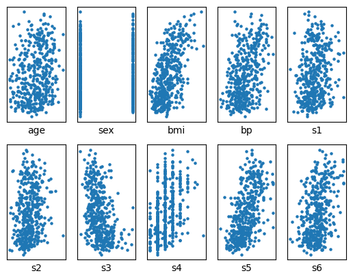
# Decide which features are useful for predicting the disease progression
# Feature engineering (Week 5 for through explanation)
bp = diabetes_X[:,3]
s5 = diabetes_X[:,8]
diabetes_X = np.array([bp,s5]).T
Split the data into a training set and a test set
Typically you do not want to train the machine learning model on the entire data set. Rather, you want to train the model on most of the data but reserve some of the original data set to test the model’s performance.
train_test_split from Scikit-Learn is a common way to randomly split a data set into a training set and a test set.
X_train, X_test, y_train, y_test = train_test_split(diabetes_X, diabetes_y, test_size=0.2)Train the machine learning algorithm with the training set
# Create linear regression object
linear_regression = LinearRegression()

# Train the model using the training sets
linear_regression.fit(X_train, y_train)LinearRegression()In a Jupyter environment, please rerun this cell to show the HTML representation or trust the notebook.
On GitHub, the HTML representation is unable to render, please try loading this page with nbviewer.org.
LinearRegression()
Test the performance of the trained model with the test set using numerical metrics and visual analysis
# Make predictions using the testing set
y_pred = linear_regression.predict(X_test)
# The coefficients
print("Coefficients:", linear_regression.coef_, linear_regression.intercept_)
print()
# The mean squared error
print("Mean squared error: %.2f" % mean_squared_error(y_test, y_pred))
print("Root mean squared error: %.2f" % np.sqrt(mean_squared_error(y_test, y_pred)))
print()
# The coefficient of determination (r2 score): 1 is perfect prediction
print("R2-Score: %.2f" % r2_score(y_test, y_pred))
print()
# Percent error (absolute)
percent_error = np.average(np.abs(y_test-y_pred)/y_test)*100
print("Absolute Percent Error: %.2f" % percent_error)Coefficients: [418.64607627 773.51831138] 152.12471014987497
Mean squared error: 4980.74
Root mean squared error: 70.57
R2-Score: 0.31
Absolute Percent Error: 51.55# Plot outputs
plt.scatter(X_test[:,0], y_test, color="red", label="True")
plt.scatter(X_test[:,0], y_pred, color="blue", label="Predicted")
plt.legend()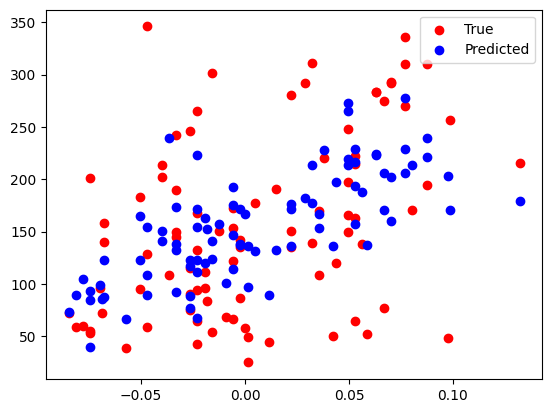
(Optional) Improve the performance of the algorithm by either reformatting the data OR changing the parameters of the machine learning algorithm
- Choose different features or a different number of features?
- Choose a different amount of test data (i.e. train the model with more data)?
- Use a different machine learning algorithm?
- Use a design matrix (Pre-Class and In-Class Assignment)?