Creating Neural Networks with Scikit-Learn and Keras

CSC/DSC 340 Week 7 Slides (Part 2)

Date Created: September 28, 2023

Last Modified: September 28, 2023

The Data Set

In this notebook, we will be attempting to use neural networks to classify the iris data set using both Scikit-Learn and Keras libraries

##############################
##          IMPORTS         ##
##############################
import numpy as np
import pandas as pd
import seaborn as sns
import matplotlib.pyplot as plt
from sklearn.datasets import load_iris

# Load the iris dataset from sklearn
iris = load_iris()

# Convert the iris dataset to a pandas dataframe
iris_data = pd.DataFrame(iris.data, columns=iris.feature_names)

# Add the target variable to the dataframe
iris_data['target'] = iris.target

sns.pairplot(iris_data, hue='target')

/Users/butlerju/Library/Python/3.9/lib/python/site-packages/seaborn/axisgrid.py:118: UserWarning: The figure layout has changed to tight
  self._figure.tight_layout(*args, **kwargs)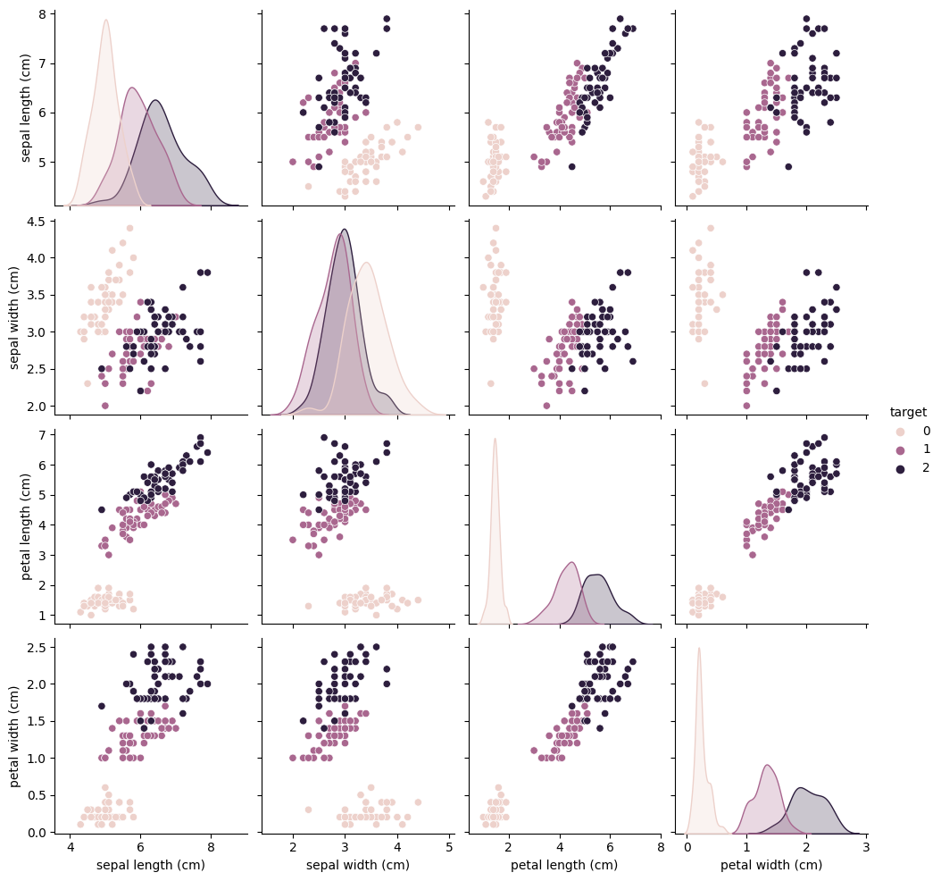

Neural Networks in Scikit-Learn with Hyperparameter Tuning

Scikit-Learn does have neural network implementations but they are called MLPClassifier (for classification problems) and MLPRegressor (for regression problems).
MLP stands for multi-layer perceptron and is another name for a simple feedforward neural network

##############################
##          IMPORTS         ##
##############################
from sklearn.model_selection import train_test_split
from sklearn.preprocessing import StandardScaler
from sklearn.neural_network import MLPClassifier
from sklearn.metrics import accuracy_score

# Load the Iris dataset
X,y = load_iris(return_X_y=True)

# Split the dataset into training and testing sets
X_train, X_test, y_train, y_test = train_test_split(X, y, test_size=0.2)

Scaling/standardizing the data is optional with neural networks but its a good thing to test to optimize the performance
Its also a good idea to explore PCA and feature engineering during this point of the notebook

# Standardize the feature values (mean=0, std=1)
scaler = StandardScaler()
X_train = scaler.fit_transform(X_train)
X_test = scaler.transform(X_test)

Define the neural network with two hidden layers, the first having 3 neurons and the second having 2 neurons.
The network will train for a maximum of 1,000 iterations or until the change between iterations is less than \(1x10^{-4}\) (whichever happens first)
Note that Scikit-Learn only allows for the activation function to be set for the entire network, not per layer
- Rectified linear unit (ReLU) by default

# Create an MLP classifier
mlp = MLPClassifier(hidden_layer_sizes=(3, 2), max_iter=1000)

Fit/train the neural network

# Train the classifier on the training data
mlp.fit(X_train, y_train)

/Users/butlerju/Library/Python/3.9/lib/python/site-packages/sklearn/neural_network/_multilayer_perceptron.py:691: ConvergenceWarning: Stochastic Optimizer: Maximum iterations (1000) reached and the optimization hasn't converged yet.
  warnings.warn(

MLPClassifier(hidden_layer_sizes=(3, 2), max_iter=1000)

In a Jupyter environment, please rerun this cell to show the HTML representation or trust the notebook.
On GitHub, the HTML representation is unable to render, please try loading this page with nbviewer.org.

Predict the classes with the trained model and test the accuracy of the trained model

# Predict the labels for the test set
y_pred = mlp.predict(X_test)

# Calculate accuracy
accuracy = accuracy_score(y_test, y_pred)
print("Accuracy:", accuracy)

Accuracy: 0.5333333333333333

We can also extract the probabilities for each category. The predict_proba method will return a list with a length equal to the number of points in the test set and the number of columns is equal to the number of classes.
The column with the highest value for a point corresponds to the most likely class the point will belong to

# Predict the probabilities for the test set
probabilities = mlp.predict_proba(X_test)

# You can print the probabilities for the first few samples as an example
print("Probabilities for the first 5 samples:")
print(probabilities[:5])

Probabilities for the first 5 samples:
[[0.06029434 0.47087469 0.46883097]
 [0.06029434 0.47087469 0.46883097]
 [0.07513704 0.49996246 0.4249005 ]
 [0.06029434 0.47087469 0.46883097]
 [0.06029434 0.47087469 0.46883097]]

Since MLPClassifier is a function within the Scikit-Learn library, its parameters can be tuned using GridSearchCV or RandomizedSearchCV

from sklearn.model_selection import RandomizedSearchCV

# Create an MLP classifier
mlp = MLPClassifier(max_iter=100000)

# Define a hyperparameter grid to search over
param_dist = {
    'hidden_layer_sizes': [(3,2), (3,3,3), (5,5,5), (2,2,2,2)],
    'activation': ['identity', 'logistic', 'tanh', 'relu'],
    'alpha': np.logspace(-15,4,500),
    'learning_rate_init': np.logspace(-15,4,500),
}

# Create RandomizedSearchCV object
random_search = RandomizedSearchCV(mlp, param_distributions=param_dist, n_iter=100, cv=5)

# Fit the RandomizedSearchCV to the training data
random_search.fit(X_train, y_train)

/Users/butlerju/Library/Python/3.9/lib/python/site-packages/sklearn/neural_network/_multilayer_perceptron.py:691: ConvergenceWarning: Stochastic Optimizer: Maximum iterations (100000) reached and the optimization hasn't converged yet.
  warnings.warn(
/Users/butlerju/Library/Python/3.9/lib/python/site-packages/sklearn/neural_network/_multilayer_perceptron.py:691: ConvergenceWarning: Stochastic Optimizer: Maximum iterations (100000) reached and the optimization hasn't converged yet.
  warnings.warn(
/Users/butlerju/Library/Python/3.9/lib/python/site-packages/sklearn/neural_network/_multilayer_perceptron.py:691: ConvergenceWarning: Stochastic Optimizer: Maximum iterations (100000) reached and the optimization hasn't converged yet.
  warnings.warn(
/Users/butlerju/Library/Python/3.9/lib/python/site-packages/sklearn/neural_network/_multilayer_perceptron.py:691: ConvergenceWarning: Stochastic Optimizer: Maximum iterations (100000) reached and the optimization hasn't converged yet.
  warnings.warn(
/Users/butlerju/Library/Python/3.9/lib/python/site-packages/sklearn/neural_network/_multilayer_perceptron.py:691: ConvergenceWarning: Stochastic Optimizer: Maximum iterations (100000) reached and the optimization hasn't converged yet.
  warnings.warn(

RandomizedSearchCV(cv=5, estimator=MLPClassifier(max_iter=100000), n_iter=100,
                   param_distributions={'activation': ['identity', 'logistic',
                                                       'tanh', 'relu'],
                                        'alpha': array([1.00000000e-15, 1.09163173e-15, 1.19165984e-15, 1.30085370e-15,
       1.42005318e-15, 1.55017512e-15, 1.69222035e-15, 1.84728144e-15,
       2.01655104e-15, 2.20133111e-15, 2.40304289e-15, 2.62323788e-15,
       2.86360...
       1.33121590e+03, 1.45319752e+03, 1.58635653e+03, 1.73171713e+03,
       1.89039738e+03, 2.06361777e+03, 2.25271064e+03, 2.45913043e+03,
       2.68446481e+03, 2.93044698e+03, 3.19896892e+03, 3.49209598e+03,
       3.81208280e+03, 4.16139055e+03, 4.54270599e+03, 4.95896201e+03,
       5.41336030e+03, 5.90939590e+03, 6.45088409e+03, 7.04198979e+03,
       7.68725952e+03, 8.39165644e+03, 9.16059848e+03, 1.00000000e+04])})

# Print the best hyperparameters
print("Best Hyperparameters:", random_search.best_params_)

Best Hyperparameters: {'learning_rate_init': 0.0007581576457522118, 'hidden_layer_sizes': (3, 3, 3), 'alpha': 0.4563716281924773, 'activation': 'identity'}

# Get the best model
best_mlp = random_search.best_estimator_

# Predict the labels for the test set
y_pred = best_mlp.predict(X_test)

# Calculate accuracy
accuracy = accuracy_score(y_test, y_pred)
print("Accuracy:", accuracy)

Accuracy: 1.0

Neural Networks in Keras

Keras is a machine learning library which primarily handles various types of neural networks and provides greater flexibity in construction than Scikit-Learn
Keras is built on top of another library called Tensorflow that we will learn about next week

from keras.models import Sequential
from keras.layers import Dense
from keras.utils import to_categorical

/Users/butlerju/Library/Python/3.9/lib/python/site-packages/urllib3/__init__.py:34: NotOpenSSLWarning: urllib3 v2.0 only supports OpenSSL 1.1.1+, currently the 'ssl' module is compiled with 'LibreSSL 2.8.3'. See: https://github.com/urllib3/urllib3/issues/3020
  warnings.warn(

# Load the Iris dataset
iris = load_iris()
X = iris.data
y = iris.target

# Split the dataset into training and testing sets
X_train, X_test, y_train, y_test = train_test_split(X, y, test_size=0.2)

# Standardize the feature values (mean=0, std=1)
scaler = StandardScaler()
X_train = scaler.fit_transform(X_train)
X_test = scaler.transform(X_test)

As an extra preprocessing step, we need to covert the data from categorical to binary vectors using the one-hot encoding processs and the Keras function to_categorical

# Convert labels to one-hot encoding
y_train = to_categorical(y_train, num_classes=3)
y_test = to_categorical(y_test, num_classes=3)

We are going to create a sequential model which will let us add layers from the first layer to the last in order

# Create a Sequential model
model = Sequential()

Add the first hidden layer to the model with 8 neurons and a relu activation function
We also have to set the input dimensio (4 in this case) when we add the first hudden layer to the model

# Add an input layer with 4 input nodes (features)
model.add(Dense(8, input_dim=4, activation='relu'))

Add a second hidden layer with 8 neurons and a relu activation function

# Add a hidden layer with 8 nodes and ReLU activation
model.add(Dense(8, activation='relu'))

Add a final layer (the output layer) which has the appropriate dimension (the number of classes with one-hot encoding) and a softmax activation function
Softmax is a popular activation function for the output layer when doing classification
- Gives probabilities and is useful in multiclass problems

# Add an output layer with 3 nodes (one for each class) and softmax activation
model.add(Dense(3, activation='softmax'))

Compile the model using a categorical cross-entropy loss function, and Adam optimizer, and using accuracy as the training and prediction metric since this is a classification problem

# Compile the model
model.compile(loss='categorical_crossentropy', optimizer='adam', metrics=['accuracy'])

Fit/train the model using 100 training iterations
verbose = 1 prints the loss and accuracy per epoch

# Train the model
model.fit(X_train, y_train, epochs=100,verbose=1)

Epoch 1/100
4/4 [==============================] - 0s 1ms/step - loss: 0.8906 - accuracy: 0.6250
Epoch 2/100
4/4 [==============================] - 0s 1ms/step - loss: 0.8733 - accuracy: 0.6250
Epoch 3/100
4/4 [==============================] - 0s 1ms/step - loss: 0.8570 - accuracy: 0.6250
Epoch 4/100
4/4 [==============================] - 0s 1ms/step - loss: 0.8418 - accuracy: 0.6250
Epoch 5/100
4/4 [==============================] - 0s 977us/step - loss: 0.8268 - accuracy: 0.6333
Epoch 6/100
4/4 [==============================] - 0s 1ms/step - loss: 0.8121 - accuracy: 0.6417
Epoch 7/100
4/4 [==============================] - 0s 1ms/step - loss: 0.7998 - accuracy: 0.6500
Epoch 8/100
4/4 [==============================] - 0s 1ms/step - loss: 0.7863 - accuracy: 0.6583
Epoch 9/100
4/4 [==============================] - 0s 1ms/step - loss: 0.7742 - accuracy: 0.6667
Epoch 10/100
4/4 [==============================] - 0s 929us/step - loss: 0.7619 - accuracy: 0.6750
Epoch 11/100
4/4 [==============================] - 0s 916us/step - loss: 0.7511 - accuracy: 0.6917
Epoch 12/100
4/4 [==============================] - 0s 1ms/step - loss: 0.7399 - accuracy: 0.6917
Epoch 13/100
4/4 [==============================] - 0s 1ms/step - loss: 0.7290 - accuracy: 0.7250
Epoch 14/100
4/4 [==============================] - 0s 1ms/step - loss: 0.7185 - accuracy: 0.7333
Epoch 15/100
4/4 [==============================] - 0s 974us/step - loss: 0.7083 - accuracy: 0.7333
Epoch 16/100
4/4 [==============================] - 0s 957us/step - loss: 0.6984 - accuracy: 0.7583
Epoch 17/100
4/4 [==============================] - 0s 970us/step - loss: 0.6885 - accuracy: 0.7583
Epoch 18/100
4/4 [==============================] - 0s 914us/step - loss: 0.6789 - accuracy: 0.7583
Epoch 19/100
4/4 [==============================] - 0s 977us/step - loss: 0.6694 - accuracy: 0.7833
Epoch 20/100
4/4 [==============================] - 0s 1ms/step - loss: 0.6601 - accuracy: 0.8000
Epoch 21/100
4/4 [==============================] - 0s 1ms/step - loss: 0.6506 - accuracy: 0.8083
Epoch 22/100
4/4 [==============================] - 0s 925us/step - loss: 0.6413 - accuracy: 0.8083
Epoch 23/100
4/4 [==============================] - 0s 919us/step - loss: 0.6321 - accuracy: 0.8083
Epoch 24/100
4/4 [==============================] - 0s 813us/step - loss: 0.6225 - accuracy: 0.8083
Epoch 25/100
4/4 [==============================] - 0s 1ms/step - loss: 0.6134 - accuracy: 0.8000
Epoch 26/100
4/4 [==============================] - 0s 1ms/step - loss: 0.6041 - accuracy: 0.8000
Epoch 27/100
4/4 [==============================] - 0s 807us/step - loss: 0.5952 - accuracy: 0.8167
Epoch 28/100
4/4 [==============================] - 0s 946us/step - loss: 0.5862 - accuracy: 0.8250
Epoch 29/100
4/4 [==============================] - 0s 960us/step - loss: 0.5768 - accuracy: 0.8250
Epoch 30/100
4/4 [==============================] - 0s 923us/step - loss: 0.5677 - accuracy: 0.8250
Epoch 31/100
4/4 [==============================] - 0s 1ms/step - loss: 0.5590 - accuracy: 0.8417
Epoch 32/100
4/4 [==============================] - 0s 970us/step - loss: 0.5500 - accuracy: 0.8417
Epoch 33/100
4/4 [==============================] - 0s 1ms/step - loss: 0.5414 - accuracy: 0.8500
Epoch 34/100
4/4 [==============================] - 0s 1ms/step - loss: 0.5326 - accuracy: 0.8500
Epoch 35/100
4/4 [==============================] - 0s 933us/step - loss: 0.5237 - accuracy: 0.8500
Epoch 36/100
4/4 [==============================] - 0s 895us/step - loss: 0.5151 - accuracy: 0.8500
Epoch 37/100
4/4 [==============================] - 0s 894us/step - loss: 0.5062 - accuracy: 0.8583
Epoch 38/100
4/4 [==============================] - 0s 1ms/step - loss: 0.4971 - accuracy: 0.8583
Epoch 39/100
4/4 [==============================] - 0s 868us/step - loss: 0.4878 - accuracy: 0.8667
Epoch 40/100
4/4 [==============================] - 0s 810us/step - loss: 0.4792 - accuracy: 0.8667
Epoch 41/100
4/4 [==============================] - 0s 862us/step - loss: 0.4708 - accuracy: 0.8667
Epoch 42/100
4/4 [==============================] - 0s 994us/step - loss: 0.4623 - accuracy: 0.8750
Epoch 43/100
4/4 [==============================] - 0s 904us/step - loss: 0.4545 - accuracy: 0.8750
Epoch 44/100
4/4 [==============================] - 0s 1ms/step - loss: 0.4460 - accuracy: 0.8833
Epoch 45/100
4/4 [==============================] - 0s 902us/step - loss: 0.4382 - accuracy: 0.8833
Epoch 46/100
4/4 [==============================] - 0s 996us/step - loss: 0.4301 - accuracy: 0.8833
Epoch 47/100
4/4 [==============================] - 0s 975us/step - loss: 0.4223 - accuracy: 0.8833
Epoch 48/100
4/4 [==============================] - 0s 2ms/step - loss: 0.4148 - accuracy: 0.8833
Epoch 49/100
4/4 [==============================] - 0s 1ms/step - loss: 0.4072 - accuracy: 0.8833
Epoch 50/100
4/4 [==============================] - 0s 889us/step - loss: 0.3998 - accuracy: 0.8833
Epoch 51/100
4/4 [==============================] - 0s 980us/step - loss: 0.3927 - accuracy: 0.8833
Epoch 52/100
4/4 [==============================] - 0s 972us/step - loss: 0.3856 - accuracy: 0.8917
Epoch 53/100
4/4 [==============================] - 0s 920us/step - loss: 0.3787 - accuracy: 0.9000
Epoch 54/100
4/4 [==============================] - 0s 836us/step - loss: 0.3717 - accuracy: 0.9083
Epoch 55/100
4/4 [==============================] - 0s 975us/step - loss: 0.3651 - accuracy: 0.9083
Epoch 56/100
4/4 [==============================] - 0s 955us/step - loss: 0.3584 - accuracy: 0.9167
Epoch 57/100
4/4 [==============================] - 0s 869us/step - loss: 0.3518 - accuracy: 0.9250
Epoch 58/100
4/4 [==============================] - 0s 967us/step - loss: 0.3458 - accuracy: 0.9250
Epoch 59/100
4/4 [==============================] - 0s 1ms/step - loss: 0.3391 - accuracy: 0.9333
Epoch 60/100
4/4 [==============================] - 0s 891us/step - loss: 0.3330 - accuracy: 0.9333
Epoch 61/100
4/4 [==============================] - 0s 948us/step - loss: 0.3273 - accuracy: 0.9333
Epoch 62/100
4/4 [==============================] - 0s 1ms/step - loss: 0.3215 - accuracy: 0.9333
Epoch 63/100
4/4 [==============================] - 0s 937us/step - loss: 0.3159 - accuracy: 0.9333
Epoch 64/100
4/4 [==============================] - 0s 900us/step - loss: 0.3101 - accuracy: 0.9333
Epoch 65/100
4/4 [==============================] - 0s 1ms/step - loss: 0.3049 - accuracy: 0.9333
Epoch 66/100
4/4 [==============================] - 0s 1ms/step - loss: 0.2996 - accuracy: 0.9333
Epoch 67/100
4/4 [==============================] - 0s 890us/step - loss: 0.2944 - accuracy: 0.9333
Epoch 68/100
4/4 [==============================] - 0s 945us/step - loss: 0.2896 - accuracy: 0.9333
Epoch 69/100
4/4 [==============================] - 0s 919us/step - loss: 0.2848 - accuracy: 0.9333
Epoch 70/100
4/4 [==============================] - 0s 915us/step - loss: 0.2798 - accuracy: 0.9333
Epoch 71/100
4/4 [==============================] - 0s 864us/step - loss: 0.2755 - accuracy: 0.9250
Epoch 72/100
4/4 [==============================] - 0s 1ms/step - loss: 0.2712 - accuracy: 0.9417
Epoch 73/100
4/4 [==============================] - 0s 876us/step - loss: 0.2666 - accuracy: 0.9500
Epoch 74/100
4/4 [==============================] - 0s 897us/step - loss: 0.2619 - accuracy: 0.9500
Epoch 75/100
4/4 [==============================] - 0s 1ms/step - loss: 0.2578 - accuracy: 0.9417
Epoch 76/100
4/4 [==============================] - 0s 889us/step - loss: 0.2538 - accuracy: 0.9417
Epoch 77/100
4/4 [==============================] - 0s 858us/step - loss: 0.2497 - accuracy: 0.9417
Epoch 78/100
4/4 [==============================] - 0s 813us/step - loss: 0.2460 - accuracy: 0.9417
Epoch 79/100
4/4 [==============================] - 0s 1ms/step - loss: 0.2420 - accuracy: 0.9417
Epoch 80/100
4/4 [==============================] - 0s 821us/step - loss: 0.2383 - accuracy: 0.9417
Epoch 81/100
4/4 [==============================] - 0s 852us/step - loss: 0.2346 - accuracy: 0.9500
Epoch 82/100
4/4 [==============================] - 0s 967us/step - loss: 0.2311 - accuracy: 0.9500
Epoch 83/100
4/4 [==============================] - 0s 1ms/step - loss: 0.2274 - accuracy: 0.9500
Epoch 84/100
4/4 [==============================] - 0s 1ms/step - loss: 0.2242 - accuracy: 0.9500
Epoch 85/100
4/4 [==============================] - 0s 1ms/step - loss: 0.2206 - accuracy: 0.9500
Epoch 86/100
4/4 [==============================] - 0s 1ms/step - loss: 0.2170 - accuracy: 0.9500
Epoch 87/100
4/4 [==============================] - 0s 1ms/step - loss: 0.2136 - accuracy: 0.9500
Epoch 88/100
4/4 [==============================] - 0s 844us/step - loss: 0.2100 - accuracy: 0.9500
Epoch 89/100
4/4 [==============================] - 0s 938us/step - loss: 0.2064 - accuracy: 0.9500
Epoch 90/100
4/4 [==============================] - 0s 833us/step - loss: 0.2029 - accuracy: 0.9500
Epoch 91/100
4/4 [==============================] - 0s 804us/step - loss: 0.1996 - accuracy: 0.9500
Epoch 92/100
4/4 [==============================] - 0s 851us/step - loss: 0.1963 - accuracy: 0.9500
Epoch 93/100
4/4 [==============================] - 0s 835us/step - loss: 0.1932 - accuracy: 0.9500
Epoch 94/100
4/4 [==============================] - 0s 833us/step - loss: 0.1901 - accuracy: 0.9500
Epoch 95/100
4/4 [==============================] - 0s 853us/step - loss: 0.1866 - accuracy: 0.9583
Epoch 96/100
4/4 [==============================] - 0s 1ms/step - loss: 0.1837 - accuracy: 0.9583
Epoch 97/100
4/4 [==============================] - 0s 852us/step - loss: 0.1807 - accuracy: 0.9583
Epoch 98/100
4/4 [==============================] - 0s 812us/step - loss: 0.1778 - accuracy: 0.9583
Epoch 99/100
4/4 [==============================] - 0s 808us/step - loss: 0.1751 - accuracy: 0.9583
Epoch 100/100
4/4 [==============================] - 0s 2ms/step - loss: 0.1724 - accuracy: 0.9667

<keras.src.callbacks.History at 0x16b2baac0>

We can then evaluate the performance of the model, both in terms of loss (not particularly helpful unless you understand the loss function values) and in terms of the accuracy

# Evaluate the model on the test set
loss, accuracy = model.evaluate(X_test, y_test)
print("Test Loss:", loss)
print("Test Accuracy:", accuracy)

1/1 [==============================] - 0s 59ms/step - loss: 0.1886 - accuracy: 0.9667
Test Loss: 0.18863752484321594
Test Accuracy: 0.9666666388511658

It is relatively common to build the Keras model in a function that returns the model so the model is easy to edit and reuse

def iris_classification_model ():
    # Create a Sequential model
    model = Sequential()

    # Add an input layer with 4 input nodes (features)
    model.add(Dense(8, input_dim=4, activation='relu'))

    # Add a hidden layer with 8 nodes and ReLU activation
    model.add(Dense(8, activation='relu'))

    # Add an output layer with 3 nodes (one for each class) and softmax activation
    model.add(Dense(3, activation='softmax'))

    # Compile the model
    model.compile(loss='categorical_crossentropy', optimizer='adam', metrics=['accuracy'])
    
    return model

model = iris_classification_model()

# Train the model
model.fit(X_train, y_train, epochs=100,verbose=1)

# Evaluate the model on the test set
loss, accuracy = model.evaluate(X_test, y_test)
print("Test Loss:", loss)
print("Test Accuracy:", accuracy)

Epoch 1/100
4/4 [==============================] - 0s 1ms/step - loss: 1.2004 - accuracy: 0.3917
Epoch 2/100
4/4 [==============================] - 0s 964us/step - loss: 1.1747 - accuracy: 0.4417
Epoch 3/100
4/4 [==============================] - 0s 937us/step - loss: 1.1525 - accuracy: 0.4833
Epoch 4/100
4/4 [==============================] - 0s 1ms/step - loss: 1.1298 - accuracy: 0.5167
Epoch 5/100
4/4 [==============================] - 0s 1ms/step - loss: 1.1084 - accuracy: 0.5250
Epoch 6/100
4/4 [==============================] - 0s 1ms/step - loss: 1.0884 - accuracy: 0.5250
Epoch 7/100
4/4 [==============================] - 0s 1ms/step - loss: 1.0693 - accuracy: 0.5333
Epoch 8/100
4/4 [==============================] - 0s 927us/step - loss: 1.0501 - accuracy: 0.5417
Epoch 9/100
4/4 [==============================] - 0s 958us/step - loss: 1.0322 - accuracy: 0.5417
Epoch 10/100
4/4 [==============================] - 0s 1ms/step - loss: 1.0144 - accuracy: 0.5500
Epoch 11/100
4/4 [==============================] - 0s 924us/step - loss: 0.9981 - accuracy: 0.5583
Epoch 12/100
4/4 [==============================] - 0s 1ms/step - loss: 0.9819 - accuracy: 0.5583
Epoch 13/100
4/4 [==============================] - 0s 904us/step - loss: 0.9658 - accuracy: 0.5500
Epoch 14/100
4/4 [==============================] - 0s 989us/step - loss: 0.9501 - accuracy: 0.5583
Epoch 15/100
4/4 [==============================] - 0s 895us/step - loss: 0.9338 - accuracy: 0.5583
Epoch 16/100
4/4 [==============================] - 0s 852us/step - loss: 0.9187 - accuracy: 0.5667
Epoch 17/100
4/4 [==============================] - 0s 876us/step - loss: 0.9028 - accuracy: 0.5667
Epoch 18/100
4/4 [==============================] - 0s 1ms/step - loss: 0.8877 - accuracy: 0.5667
Epoch 19/100
4/4 [==============================] - 0s 978us/step - loss: 0.8719 - accuracy: 0.5667
Epoch 20/100
4/4 [==============================] - 0s 884us/step - loss: 0.8571 - accuracy: 0.5833
Epoch 21/100
4/4 [==============================] - 0s 1ms/step - loss: 0.8423 - accuracy: 0.5917
Epoch 22/100
4/4 [==============================] - 0s 912us/step - loss: 0.8281 - accuracy: 0.5917
Epoch 23/100
4/4 [==============================] - 0s 1ms/step - loss: 0.8146 - accuracy: 0.6000
Epoch 24/100
4/4 [==============================] - 0s 963us/step - loss: 0.8016 - accuracy: 0.6667
Epoch 25/100
4/4 [==============================] - 0s 848us/step - loss: 0.7898 - accuracy: 0.6667
Epoch 26/100
4/4 [==============================] - 0s 837us/step - loss: 0.7778 - accuracy: 0.6750
Epoch 27/100
4/4 [==============================] - 0s 821us/step - loss: 0.7664 - accuracy: 0.6917
Epoch 28/100
4/4 [==============================] - 0s 1ms/step - loss: 0.7562 - accuracy: 0.7000
Epoch 29/100
4/4 [==============================] - 0s 836us/step - loss: 0.7457 - accuracy: 0.7083
Epoch 30/100
4/4 [==============================] - 0s 837us/step - loss: 0.7354 - accuracy: 0.7083
Epoch 31/100
4/4 [==============================] - 0s 878us/step - loss: 0.7258 - accuracy: 0.7083
Epoch 32/100
4/4 [==============================] - 0s 795us/step - loss: 0.7161 - accuracy: 0.7333
Epoch 33/100
4/4 [==============================] - 0s 1ms/step - loss: 0.7069 - accuracy: 0.7750
Epoch 34/100
4/4 [==============================] - 0s 896us/step - loss: 0.6978 - accuracy: 0.7750
Epoch 35/100
4/4 [==============================] - 0s 1ms/step - loss: 0.6890 - accuracy: 0.7917
Epoch 36/100
4/4 [==============================] - 0s 953us/step - loss: 0.6802 - accuracy: 0.8083
Epoch 37/100
4/4 [==============================] - 0s 859us/step - loss: 0.6714 - accuracy: 0.8167
Epoch 38/100
4/4 [==============================] - 0s 942us/step - loss: 0.6631 - accuracy: 0.8250
Epoch 39/100
4/4 [==============================] - 0s 914us/step - loss: 0.6550 - accuracy: 0.8250
Epoch 40/100
4/4 [==============================] - 0s 844us/step - loss: 0.6469 - accuracy: 0.8333
Epoch 41/100
4/4 [==============================] - 0s 900us/step - loss: 0.6391 - accuracy: 0.8333
Epoch 42/100
4/4 [==============================] - 0s 898us/step - loss: 0.6311 - accuracy: 0.8417
Epoch 43/100
4/4 [==============================] - 0s 833us/step - loss: 0.6236 - accuracy: 0.8417
Epoch 44/100
4/4 [==============================] - 0s 898us/step - loss: 0.6159 - accuracy: 0.8417
Epoch 45/100
4/4 [==============================] - 0s 832us/step - loss: 0.6084 - accuracy: 0.8583
Epoch 46/100
4/4 [==============================] - 0s 1ms/step - loss: 0.6014 - accuracy: 0.8667
Epoch 47/100
4/4 [==============================] - 0s 825us/step - loss: 0.5941 - accuracy: 0.8667
Epoch 48/100
4/4 [==============================] - 0s 802us/step - loss: 0.5870 - accuracy: 0.8667
Epoch 49/100
4/4 [==============================] - 0s 833us/step - loss: 0.5799 - accuracy: 0.8750
Epoch 50/100
4/4 [==============================] - 0s 1ms/step - loss: 0.5732 - accuracy: 0.8750
Epoch 51/100
4/4 [==============================] - 0s 933us/step - loss: 0.5664 - accuracy: 0.8750
Epoch 52/100
4/4 [==============================] - 0s 1ms/step - loss: 0.5595 - accuracy: 0.8750
Epoch 53/100
4/4 [==============================] - 0s 920us/step - loss: 0.5532 - accuracy: 0.8833
Epoch 54/100
4/4 [==============================] - 0s 848us/step - loss: 0.5464 - accuracy: 0.8833
Epoch 55/100
4/4 [==============================] - 0s 857us/step - loss: 0.5399 - accuracy: 0.8833
Epoch 56/100
4/4 [==============================] - 0s 924us/step - loss: 0.5333 - accuracy: 0.8833
Epoch 57/100
4/4 [==============================] - 0s 898us/step - loss: 0.5271 - accuracy: 0.8833
Epoch 58/100
4/4 [==============================] - 0s 920us/step - loss: 0.5209 - accuracy: 0.8833
Epoch 59/100
4/4 [==============================] - 0s 824us/step - loss: 0.5145 - accuracy: 0.8833
Epoch 60/100
4/4 [==============================] - 0s 896us/step - loss: 0.5079 - accuracy: 0.8833
Epoch 61/100
4/4 [==============================] - 0s 875us/step - loss: 0.5016 - accuracy: 0.9000
Epoch 62/100
4/4 [==============================] - 0s 824us/step - loss: 0.4954 - accuracy: 0.9000
Epoch 63/100
4/4 [==============================] - 0s 859us/step - loss: 0.4892 - accuracy: 0.9000
Epoch 64/100
4/4 [==============================] - 0s 830us/step - loss: 0.4828 - accuracy: 0.9000
Epoch 65/100
4/4 [==============================] - 0s 952us/step - loss: 0.4769 - accuracy: 0.9083
Epoch 66/100
4/4 [==============================] - 0s 981us/step - loss: 0.4707 - accuracy: 0.9083
Epoch 67/100
4/4 [==============================] - 0s 892us/step - loss: 0.4643 - accuracy: 0.9083
Epoch 68/100
4/4 [==============================] - 0s 902us/step - loss: 0.4585 - accuracy: 0.9083
Epoch 69/100
4/4 [==============================] - 0s 973us/step - loss: 0.4527 - accuracy: 0.9000
Epoch 70/100
4/4 [==============================] - 0s 943us/step - loss: 0.4468 - accuracy: 0.9000
Epoch 71/100
4/4 [==============================] - 0s 861us/step - loss: 0.4408 - accuracy: 0.9000
Epoch 72/100
4/4 [==============================] - 0s 868us/step - loss: 0.4349 - accuracy: 0.9000
Epoch 73/100
4/4 [==============================] - 0s 877us/step - loss: 0.4293 - accuracy: 0.8917
Epoch 74/100
4/4 [==============================] - 0s 814us/step - loss: 0.4230 - accuracy: 0.8917
Epoch 75/100
4/4 [==============================] - 0s 1ms/step - loss: 0.4176 - accuracy: 0.8917
Epoch 76/100
4/4 [==============================] - 0s 885us/step - loss: 0.4115 - accuracy: 0.8917
Epoch 77/100
4/4 [==============================] - 0s 813us/step - loss: 0.4059 - accuracy: 0.9000
Epoch 78/100
4/4 [==============================] - 0s 771us/step - loss: 0.4002 - accuracy: 0.9000
Epoch 79/100
4/4 [==============================] - 0s 880us/step - loss: 0.3946 - accuracy: 0.9000
Epoch 80/100
4/4 [==============================] - 0s 856us/step - loss: 0.3888 - accuracy: 0.9000
Epoch 81/100
4/4 [==============================] - 0s 874us/step - loss: 0.3833 - accuracy: 0.9000
Epoch 82/100
4/4 [==============================] - 0s 838us/step - loss: 0.3779 - accuracy: 0.9083
Epoch 83/100
4/4 [==============================] - 0s 839us/step - loss: 0.3721 - accuracy: 0.9083
Epoch 84/100
4/4 [==============================] - 0s 813us/step - loss: 0.3664 - accuracy: 0.9083
Epoch 85/100
4/4 [==============================] - 0s 833us/step - loss: 0.3612 - accuracy: 0.9083
Epoch 86/100
4/4 [==============================] - 0s 819us/step - loss: 0.3554 - accuracy: 0.9083
Epoch 87/100
4/4 [==============================] - 0s 864us/step - loss: 0.3498 - accuracy: 0.9083
Epoch 88/100
4/4 [==============================] - 0s 855us/step - loss: 0.3445 - accuracy: 0.9083
Epoch 89/100
4/4 [==============================] - 0s 808us/step - loss: 0.3392 - accuracy: 0.9083
Epoch 90/100
4/4 [==============================] - 0s 884us/step - loss: 0.3334 - accuracy: 0.9167
Epoch 91/100
4/4 [==============================] - 0s 836us/step - loss: 0.3281 - accuracy: 0.9167
Epoch 92/100
4/4 [==============================] - 0s 816us/step - loss: 0.3235 - accuracy: 0.9167
Epoch 93/100
4/4 [==============================] - 0s 820us/step - loss: 0.3176 - accuracy: 0.9167
Epoch 94/100
4/4 [==============================] - 0s 869us/step - loss: 0.3127 - accuracy: 0.9167
Epoch 95/100
4/4 [==============================] - 0s 799us/step - loss: 0.3077 - accuracy: 0.9167
Epoch 96/100
4/4 [==============================] - 0s 832us/step - loss: 0.3027 - accuracy: 0.9083
Epoch 97/100
4/4 [==============================] - 0s 1ms/step - loss: 0.2977 - accuracy: 0.9083
Epoch 98/100
4/4 [==============================] - 0s 850us/step - loss: 0.2929 - accuracy: 0.9083
Epoch 99/100
4/4 [==============================] - 0s 898us/step - loss: 0.2883 - accuracy: 0.9083
Epoch 100/100
4/4 [==============================] - 0s 850us/step - loss: 0.2831 - accuracy: 0.9083
1/1 [==============================] - 0s 50ms/step - loss: 0.2810 - accuracy: 0.9667
Test Loss: 0.28102296590805054
Test Accuracy: 0.9666666388511658

Having the model as a function allows hyperparameters to be passed as arguments which is useful for hyperparameter tuning

def iris_classification_model (neurons1, neurons2):
    # Create a Sequential model
    model = Sequential()

    # Add an input layer with 4 input nodes (features)
    model.add(Dense(neurons1, input_dim=4, activation='relu'))

    # Add a hidden layer with 8 nodes and ReLU activation
    model.add(Dense(neurons2, activation='relu'))

    # Add an output layer with 3 nodes (one for each class) and softmax activation
    model.add(Dense(3, activation='softmax'))

    # Compile the model
    model.compile(loss='categorical_crossentropy', optimizer='adam', metrics=['accuracy'])
    
    return model

You can tune a Keras model using the for loop method

for neurons1 in range(1,6):
    for neurons2 in range(1,6):
        model = iris_classification_model(neurons1, neurons2)

        # Train the model
        model.fit(X_train, y_train, epochs=100,verbose=0)
        
        # Evaluate the model on the test set
        loss, accuracy = model.evaluate(X_test, y_test)
        print("Neurons:", neurons1, neurons2)
        print("Test Accuracy:", accuracy)
        print()

1/1 [==============================] - 0s 40ms/step - loss: 1.1178 - accuracy: 0.4667
Neurons: 1 1
Test Accuracy: 0.46666666865348816

1/1 [==============================] - 0s 40ms/step - loss: 0.7348 - accuracy: 0.6333
Neurons: 1 2
Test Accuracy: 0.6333333253860474

WARNING:tensorflow:5 out of the last 5 calls to <function Model.make_test_function.<locals>.test_function at 0x16c5f9c10> triggered tf.function retracing. Tracing is expensive and the excessive number of tracings could be due to (1) creating @tf.function repeatedly in a loop, (2) passing tensors with different shapes, (3) passing Python objects instead of tensors. For (1), please define your @tf.function outside of the loop. For (2), @tf.function has reduce_retracing=True option that can avoid unnecessary retracing. For (3), please refer to https://www.tensorflow.org/guide/function#controlling_retracing and https://www.tensorflow.org/api_docs/python/tf/function for  more details.
1/1 [==============================] - 0s 41ms/step - loss: 1.1030 - accuracy: 0.2667
Neurons: 1 3
Test Accuracy: 0.2666666805744171

WARNING:tensorflow:6 out of the last 6 calls to <function Model.make_test_function.<locals>.test_function at 0x16c696ca0> triggered tf.function retracing. Tracing is expensive and the excessive number of tracings could be due to (1) creating @tf.function repeatedly in a loop, (2) passing tensors with different shapes, (3) passing Python objects instead of tensors. For (1), please define your @tf.function outside of the loop. For (2), @tf.function has reduce_retracing=True option that can avoid unnecessary retracing. For (3), please refer to https://www.tensorflow.org/guide/function#controlling_retracing and https://www.tensorflow.org/api_docs/python/tf/function for  more details.
1/1 [==============================] - 0s 43ms/step - loss: 1.1030 - accuracy: 0.2667
Neurons: 1 4
Test Accuracy: 0.2666666805744171

1/1 [==============================] - 0s 44ms/step - loss: 0.8486 - accuracy: 0.6333
Neurons: 1 5
Test Accuracy: 0.6333333253860474

1/1 [==============================] - 0s 41ms/step - loss: 0.7724 - accuracy: 0.6333
Neurons: 2 1
Test Accuracy: 0.6333333253860474

1/1 [==============================] - 0s 43ms/step - loss: 1.0671 - accuracy: 0.5333
Neurons: 2 2
Test Accuracy: 0.5333333611488342

1/1 [==============================] - 0s 40ms/step - loss: 0.7124 - accuracy: 0.7667
Neurons: 2 3
Test Accuracy: 0.7666666507720947

1/1 [==============================] - 0s 45ms/step - loss: 0.8310 - accuracy: 0.6333
Neurons: 2 4
Test Accuracy: 0.6333333253860474

1/1 [==============================] - 0s 45ms/step - loss: 0.6199 - accuracy: 0.6333
Neurons: 2 5
Test Accuracy: 0.6333333253860474

1/1 [==============================] - 0s 41ms/step - loss: 0.8380 - accuracy: 0.7000
Neurons: 3 1
Test Accuracy: 0.699999988079071

1/1 [==============================] - 0s 41ms/step - loss: 0.8543 - accuracy: 0.6333
Neurons: 3 2
Test Accuracy: 0.6333333253860474

1/1 [==============================] - 0s 41ms/step - loss: 0.5630 - accuracy: 0.7333
Neurons: 3 3
Test Accuracy: 0.7333333492279053

1/1 [==============================] - 0s 40ms/step - loss: 0.6921 - accuracy: 0.7000
Neurons: 3 4
Test Accuracy: 0.699999988079071

1/1 [==============================] - 0s 41ms/step - loss: 0.5077 - accuracy: 0.8333
Neurons: 3 5
Test Accuracy: 0.8333333134651184

1/1 [==============================] - 0s 40ms/step - loss: 0.7243 - accuracy: 0.7000
Neurons: 4 1
Test Accuracy: 0.699999988079071

1/1 [==============================] - 0s 40ms/step - loss: 0.8310 - accuracy: 0.6000
Neurons: 4 2
Test Accuracy: 0.6000000238418579

1/1 [==============================] - 0s 40ms/step - loss: 0.7262 - accuracy: 0.6333
Neurons: 4 3
Test Accuracy: 0.6333333253860474

1/1 [==============================] - 0s 40ms/step - loss: 0.7375 - accuracy: 0.7000
Neurons: 4 4
Test Accuracy: 0.699999988079071

1/1 [==============================] - 0s 41ms/step - loss: 0.5332 - accuracy: 0.8000
Neurons: 4 5
Test Accuracy: 0.800000011920929

1/1 [==============================] - 0s 41ms/step - loss: 0.7142 - accuracy: 0.6333
Neurons: 5 1
Test Accuracy: 0.6333333253860474

1/1 [==============================] - 0s 40ms/step - loss: 1.0705 - accuracy: 0.4000
Neurons: 5 2
Test Accuracy: 0.4000000059604645

1/1 [==============================] - 0s 43ms/step - loss: 0.6775 - accuracy: 0.6333
Neurons: 5 3
Test Accuracy: 0.6333333253860474

1/1 [==============================] - 0s 43ms/step - loss: 0.3456 - accuracy: 0.9667
Neurons: 5 4
Test Accuracy: 0.9666666388511658

1/1 [==============================] - 0s 41ms/step - loss: 0.4799 - accuracy: 0.6667
Neurons: 5 5
Test Accuracy: 0.6666666865348816

There are many ways to create Keras function for hyperaparameter tuning, some of which will be more general

# Define a function to create a Keras model
def create_model(hidden_layers=1, neurons=8, learning_rate=0.001):
    model = Sequential()
    model.add(Dense(neurons, input_dim=4, activation='relu'))
    
    for _ in range(hidden_layers - 1):
        model.add(Dense(neurons, activation='relu'))
    
    model.add(Dense(3, activation='softmax'))
    
    optimizer = Adam(learning_rate=learning_rate)
    model.compile(loss='categorical_crossentropy', optimizer=optimizer, metrics=['accuracy'])
    return model

Finally, we can also extract the probabilities from Keras the same way as Scikit-Learn

# Predict the probabilities for the test set
probabilities = model.predict(X_test)

# probabilities is a 2D array where each row corresponds to a sample in X_test
# and each column corresponds to the probability of that sample belonging to a specific class

# You can print the probabilities for the first few samples as an example
print("Probabilities for the first 5 samples:")
print(probabilities[:5])

1/1 [==============================] - 0s 42ms/step
Probabilities for the first 5 samples:
[[0.9644619  0.03330116 0.0022369 ]
 [0.02708035 0.32647318 0.64644647]
 [0.00750907 0.2402518  0.7522391 ]
 [0.950129   0.04601447 0.00385656]
 [0.9676701  0.03039231 0.00193762]]