Creating Neural Networks with Tensorflow

CSC/DSC 340 Week 8 Slides

Date Created: October 6, 2023

Last Modified: October 6, 2023

Keras and Tensorflow

Keras and Tensorflow use to be seperate libraries but Keras is now apart of Tensorflow
In recent versions of Tensorflow, it has become hard to create and use neural networks without also using Keras
However, there are a few features that are still useful

Keras Neural Network With New Data Set

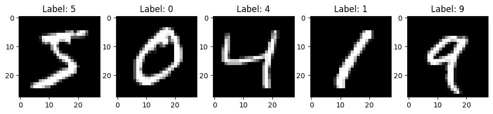
MNIST Data Set
- Input: images of handwritten digits (28x28 pixels)
- Output: digit shown in the image
We will go into more detail on image manipulation and classification when we cover neural networks, but we can do a preliminary analysis on the MNIST data set with regular neural networks.

import matplotlib.pyplot as plt
from tensorflow.keras.datasets import mnist

## NOTE: The same data set is avaliable from Scikit-Learn

/Users/butlerju/Library/Python/3.9/lib/python/site-packages/urllib3/__init__.py:34: NotOpenSSLWarning: urllib3 v2.0 only supports OpenSSL 1.1.1+, currently the 'ssl' module is compiled with 'LibreSSL 2.8.3'. See: https://github.com/urllib3/urllib3/issues/3020
  warnings.warn(

(train_images, train_labels), (test_images, test_labels) = mnist.load_data()

print(len(train_images))

# Display a few sample images
num_samples = 5  # Change this to display a different number of images

plt.figure(figsize=(12, 4))

for i in range(num_samples):
    plt.subplot(1, num_samples, i + 1)
    plt.imshow(train_images[i], cmap='gray')
    plt.title(f"Label: {train_labels[i]}")

plt.show()

import numpy as np
import tensorflow as tf
from tensorflow.keras.datasets import mnist
from tensorflow.keras.models import Sequential
from tensorflow.keras.layers import Dense
from tensorflow.keras.utils import to_categorical

# Normalize pixel values to be between 0 and 1
train_images, test_images = train_images / 255.0, test_images / 255.0

# One-hot encode the labels
train_labels = to_categorical(train_labels)
test_labels = to_categorical(test_labels)

np.shape(train_images[i])

(28, 28)

def mnist_classification_model ():
    # Define the model
    model = Sequential()

    # Add layers to the model
    model.add(Flatten(input_shape=(28, 28)))  # Flatten the 28x28 input images to a 1D vector
    model.add(Dense(128, activation='relu'))  # Fully connected layer with ReLU activation
    model.add(Dense(64, activation='relu'))   # Another fully connected layer with ReLU activation
    model.add(Dense(10, activation='softmax')) # Output layer with 10 neurons for 10 classes (digits 0-9)
    
    # Compile the model
    model.compile(optimizer='adam', loss='categorical_crossentropy', metrics=['accuracy'])
    return model

mnist_model = mnist_classification_model ()

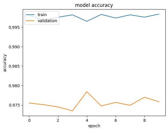
history = mnist_model.fit(train_images, train_labels, epochs=10, batch_size=32, validation_split=0.2, verbose=1)

Epoch 1/10
1500/1500 [==============================] - 1s 835us/step - loss: 0.0065 - accuracy: 0.9980 - val_loss: 0.1808 - val_accuracy: 0.9755
Epoch 2/10
1500/1500 [==============================] - 1s 828us/step - loss: 0.0098 - accuracy: 0.9969 - val_loss: 0.1679 - val_accuracy: 0.9751
Epoch 3/10
1500/1500 [==============================] - 1s 810us/step - loss: 0.0079 - accuracy: 0.9975 - val_loss: 0.1697 - val_accuracy: 0.9745
Epoch 4/10
1500/1500 [==============================] - 1s 808us/step - loss: 0.0059 - accuracy: 0.9982 - val_loss: 0.1896 - val_accuracy: 0.9735
Epoch 5/10
1500/1500 [==============================] - 1s 805us/step - loss: 0.0112 - accuracy: 0.9965 - val_loss: 0.1665 - val_accuracy: 0.9784
Epoch 6/10
1500/1500 [==============================] - 1s 808us/step - loss: 0.0052 - accuracy: 0.9983 - val_loss: 0.1901 - val_accuracy: 0.9747
Epoch 7/10
1500/1500 [==============================] - 1s 874us/step - loss: 0.0094 - accuracy: 0.9973 - val_loss: 0.1842 - val_accuracy: 0.9757
Epoch 8/10
1500/1500 [==============================] - 1s 857us/step - loss: 0.0063 - accuracy: 0.9982 - val_loss: 0.2077 - val_accuracy: 0.9749
Epoch 9/10
1500/1500 [==============================] - 1s 809us/step - loss: 0.0072 - accuracy: 0.9976 - val_loss: 0.1842 - val_accuracy: 0.9770
Epoch 10/10
1500/1500 [==============================] - 1s 838us/step - loss: 0.0053 - accuracy: 0.9984 - val_loss: 0.1975 - val_accuracy: 0.9758

# Evaluate the model on the test data
test_loss, test_accuracy = model.evaluate(test_images, test_labels)
print(f"Test accuracy: {test_accuracy * 100:.2f}%")

313/313 [==============================] - 0s 464us/step - loss: 0.0953 - accuracy: 0.9721
Test accuracy: 97.21%

# summarize history for accuracy
plt.plot(history.history['accuracy'])
plt.plot(history.history['val_accuracy'])
plt.title('model accuracy')
plt.ylabel('accuracy')
plt.xlabel('epoch')
plt.legend(['train', 'validation'], loc='upper left')
plt.show()

Custom Loss Functions

Tensorflow Variables

GPU Support

Preprocessing Layers

Flatten Layer

Normalization Layer

CategoryEncoding Layer

Image Preprocessing Layers

Saving Trained Models

Other Tensorflow Customizations

Tensorflow offers many other customizations besides the ones discussed here: * Custom Activation Functions * Custom Initialization Schemes * Custom Layers * Custom Training Loops

These are unlikely to be used in this course, but are good to know about for the future