Creating Neural Networks from Scratch

CSC/DSC 340 Week 9 Slides

Author: Dr. Julie Butler

Date Created: October 16, 2023

Last Modified: October 16, 2023

• This week we will learn how to create neural networks from scratch, using the Python library JAX to perform the optimization.
• Another common library for this task is autograd but it is no longer being maintained

Review of Neural Network Equations

• A return to Week 7 Slides

Creating a Neural Network from Scratch Using JAX

• JAX is an automatic differentiation library in Python that can find the derivative of any chunk of code it is given.
  
• If you are interested you can read more about the library here.

# IMPORTS
# Math for the ceiling function
from math import ceil
# Matplotlib for graphing capabilities
from matplotlib import pyplot as plt
# Numpy for arrays
import numpy as np
# Modules from the JAX library for creating neural networks
import jax.numpy as jnp
from jax import grad
from jax import random as npr

Generate the Data Set

Let’s keep things simple and generate a data points from a Gaussian curve. We will have our x data be evenly space between -10 and 10 and our y data be the corresponding points on a Gaussian curve.

# Let's create a data set that is just a basic Gaussian curve
X = np.linspace(-10,10,250)
y = np.exp(-X**2)

Perform a Train-Test Split

# We will split the data set into two pieces, a training data set that contains
# 80% of the total data and a test set that contains the other 20%
from sklearn.model_selection import train_test_split
train_size = 0.8
X_train, X_test, y_train, y_test = train_test_split(X, y, train_size=train_size)

Define the Neural Network

First we will define the sigmoid function as our activation function.

def sigmoid(x):
    """
        Calculates the value of the sigmoid function for 
        a given input of x
    """
    return 1. / (1. + jnp.exp(-x))

• Now we will define our neural network.
  
• Here we will be using an architecture with two hidden layers, each using the sigmoid activation function, and an output layer which does not have an activation function.
  
• Note that we do not use the bias offset in this code

def neural_network(W, x):
    """
        Inputs:
            W (a list): the weights of the neural network
            x (a float): the input value of the neural network
        Returns:
            Unnamed (a float): The output of the neural network
        Defines a neural network with one hidden layer.  The number of neurons in
        the hidden layer is the length of W[0]. The activation function is the 
        sigmoid function on the hidden layer an none on the output layer.
    """
    # Calculate the output for the neurons in the hidden layers
    hidden_layer1 = sigmoid(jnp.dot(x,W[0]))
    hidden_layer2 = sigmoid(jnp.dot(hidden_layer1, W[1]))
    # Calculate the result for the output neuron
    return jnp.dot(hidden_layer2, W[2])

Define the Loss Function

Now we need to define our loss function. For simplicity we will be using the mean-squared error loss function, which is a very common loss function for training neural networks.

def loss_function(W, x, y):
    """
        Inputs:
            W (a list): the weights of the neural network
            t (a 1D NumPy array): the times to calculate the predicted position at
        Returns:
            loss_sum (a float): The total loss over all times
        The loss function for the neural network to solve for position given 
        a function for acceleration.
    """
    # Define a variable to hold the total loss
    loss_sum = 0.
    # Loop through each individual time
    for i in range(len(x)):
        # Get the output of the neural network with the given set of weights
        nn = neural_network(W, x[i])[0][0]
        err_sqr = (nn-y[i])**2
        # Update the loss sum
        loss_sum += err_sqr
    loss_sum /= len(x)
    # Return the loss sum    
    return loss_sum

Train the Neural Network

• Finally we need to train our neural network.
  
• We will start by randomly initializing the weights of our neural network (with 25 neurons per hidden layer).

# Generate the key for the random number generator
key = npr.PRNGKey(0)
# Set the number of neurons in the hidden layer
number_hidden_neurons = 25
# Initialize the weights of the neural network with random numbers
W = [npr.normal(key,(1, number_hidden_neurons)), 
     npr.normal(key,(number_hidden_neurons,number_hidden_neurons)), 
     npr.normal(key,(number_hidden_neurons, 1))]

• We then define the parameters for the learning rate, the number of training iterations, and the threshold for stopping the training.

# Set the learning rate and the number of training iterations for the network
learning_rate = 0.01
num_training_iterations = 100
threshold = 0.0001
previous_loss = 0

• Next, we perform gradient descent to update the weights of the neural network over for the set number of training iterations, or until the loss function value converges to some set threshold.

WARNING: This cell will take a long time to run.

# Train the neural network for the specified number of iterations
# Update the weights using the learning rates
for i in range(num_training_iterations):
    print("Training Iteration:", i+1)
    current_loss = loss_function(W,X_train,y_train)
    print("Loss:", current_loss)
    print()
    # If the current loss is within a set threshold of the previous loss, stop
    # the training
    if np.abs(current_loss-previous_loss) < threshold:
        break;
    # Calculate the gradient of the loss function and then use that gradient to
    # update the weights of the neural network using the learning rate and the 
    # gradient descent optimization method
    loss_grad =  grad(loss_function)(W, X_train, y_train)
    # Update first hidden layer
    W[0] = W[0] - learning_rate * loss_grad[0]
    # Update second hidden layer
    W[1] = W[1] - learning_rate * loss_grad[1]
    # Update output layer
    W[2] = W[2] - learning_rate * loss_grad[2]
    previous_loss = current_loss

Training Iteration: 1
Loss: 5.7393837

Training Iteration: 2
Loss: 3.9249494

Training Iteration: 3
Loss: 2.7430646

Training Iteration: 4
Loss: 1.9642867

Training Iteration: 5
Loss: 1.4439908

Training Iteration: 6
Loss: 1.0908564

Training Iteration: 7
Loss: 0.8469455

Training Iteration: 8
Loss: 0.6752586

Training Iteration: 9
Loss: 0.5519808

Training Iteration: 10
Loss: 0.46164405

Training Iteration: 11
Loss: 0.39409688

Training Iteration: 12
Loss: 0.34260026

Training Iteration: 13
Loss: 0.30262083

Training Iteration: 14
Loss: 0.2710642

Training Iteration: 15
Loss: 0.24578558

Training Iteration: 16
Loss: 0.22527163

Training Iteration: 17
Loss: 0.20843603

Training Iteration: 18
Loss: 0.1944845

Training Iteration: 19
Loss: 0.18282592

Training Iteration: 20
Loss: 0.17301211

Training Iteration: 21
Loss: 0.16469756

Training Iteration: 22
Loss: 0.15761234

Training Iteration: 23
Loss: 0.1515421

Training Iteration: 24
Loss: 0.14631484

Training Iteration: 25
Loss: 0.14179125

Training Iteration: 26
Loss: 0.13785718

Training Iteration: 27
Loss: 0.13441862

Training Iteration: 28
Loss: 0.13139778

Training Iteration: 29
Loss: 0.12872973

Training Iteration: 30
Loss: 0.12636037

Training Iteration: 31
Loss: 0.12424435

Training Iteration: 32
Loss: 0.12234331

Training Iteration: 33
Loss: 0.12062525

Training Iteration: 34
Loss: 0.119062945

Training Iteration: 35
Loss: 0.1176336

Training Iteration: 36
Loss: 0.11631781

Training Iteration: 37
Loss: 0.11509922

Training Iteration: 38
Loss: 0.113963954

Training Iteration: 39
Loss: 0.11290028

Training Iteration: 40
Loss: 0.11189827

Training Iteration: 41
Loss: 0.11094945

Training Iteration: 42
Loss: 0.110046774

Training Iteration: 43
Loss: 0.10918406

Training Iteration: 44
Loss: 0.10835604

Training Iteration: 45
Loss: 0.1075586

Training Iteration: 46
Loss: 0.10678794

Training Iteration: 47
Loss: 0.10604083

Training Iteration: 48
Loss: 0.105314724

Training Iteration: 49
Loss: 0.10460715

Training Iteration: 50
Loss: 0.10391628

Training Iteration: 51
Loss: 0.103240326

Training Iteration: 52
Loss: 0.10257807

Training Iteration: 53
Loss: 0.10192816

Training Iteration: 54
Loss: 0.10128962

Training Iteration: 55
Loss: 0.10066156

Training Iteration: 56
Loss: 0.10004312

Training Iteration: 57
Loss: 0.09943377

Training Iteration: 58
Loss: 0.098832875

Training Iteration: 59
Loss: 0.098239936

Training Iteration: 60
Loss: 0.0976546

Training Iteration: 61
Loss: 0.097076416

Training Iteration: 62
Loss: 0.09650502

Training Iteration: 63
Loss: 0.09594035

Training Iteration: 64
Loss: 0.09538187

Training Iteration: 65
Loss: 0.09482949

Training Iteration: 66
Loss: 0.09428306

Training Iteration: 67
Loss: 0.09374238

Training Iteration: 68
Loss: 0.09320727

Training Iteration: 69
Loss: 0.09267756

Training Iteration: 70
Loss: 0.09215312

Training Iteration: 71
Loss: 0.091633804

Training Iteration: 72
Loss: 0.09111967

Training Iteration: 73
Loss: 0.090610415

Training Iteration: 74
Loss: 0.09010603

Training Iteration: 75
Loss: 0.08960638

Training Iteration: 76
Loss: 0.08911151

Training Iteration: 77
Loss: 0.08862111

Training Iteration: 78
Loss: 0.08813539

Training Iteration: 79
Loss: 0.087654

Training Iteration: 80
Loss: 0.087177046

Training Iteration: 81
Loss: 0.08670438

Training Iteration: 82
Loss: 0.08623596

Training Iteration: 83
Loss: 0.08577179

Training Iteration: 84
Loss: 0.08531174

Training Iteration: 85
Loss: 0.084855735

Training Iteration: 86
Loss: 0.08440378

Training Iteration: 87
Loss: 0.08395572

Training Iteration: 88
Loss: 0.08351156

Training Iteration: 89
Loss: 0.08307134

Training Iteration: 90
Loss: 0.08263482

Training Iteration: 91
Loss: 0.08220212

Training Iteration: 92
Loss: 0.08177301

Training Iteration: 93
Loss: 0.08134764

Training Iteration: 94
Loss: 0.08092584

Training Iteration: 95
Loss: 0.08050759

Training Iteration: 96
Loss: 0.080092885

Training Iteration: 97
Loss: 0.07968161

Training Iteration: 98
Loss: 0.07927379

Training Iteration: 99
Loss: 0.07886927

Training Iteration: 100
Loss: 0.078468055

Analyze the Results

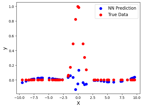
Now we need to analyze the performance of our neural network using the test data set that was reserved earlier. First we need to generate the neural network predictions for the y component of the test data set.

y_nn = [neural_network(W, xi)[0][0] for xi in X_test] 

First lets analyze the results graphically by plotting the predicted test data set and the true test data set on the same graph.

plt.scatter(X_test, y_nn, s=50, color="blue",label="NN Prediction")
plt.scatter(X_test, y_test, s=50, color="red", label="True Data")
plt.legend(fontsize=12)
plt.xlabel("X",fontsize=14)
plt.ylabel("y",fontsize=14)

Text(0, 0.5, 'y')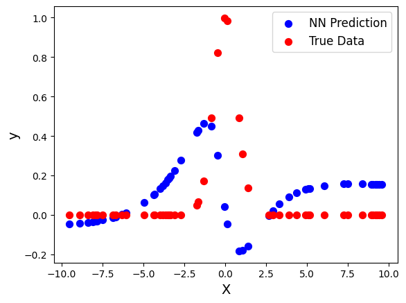

Next let’s analyze the error numerically using the root mean-squared error (RMSE) function, which is simiply the square root of the mean-squared error. The RMSE gives the average error on each data point (instead of the squared average error) so it is a met more of a clear metric for error analysis. First, let’s define a function to calculate the RMSE between two data sets.

def rmse(A,B):
    """
        Inputs:
            A,B (NumPy arrays)
        Returns:
            Unnamed (a float): the RMSE error between A and B
        Calculates the RMSE error between A and B.
    """
    assert len(A)==len(B),"The data sets must be the same length to calcualte\
        the RMSE."
    return np.sqrt(np.average((A-B)**2)) 

Now let’s print the RMSE between the true test data set and the neural network prediction.

print("RMSE between true test set and neural network result:", rmse(y_nn,y_test))

RMSE between true test set and neural network result: 0.28406674843753915

Hyperparameter Tuning: Changing the Number of Layers, the Number of Hidden Neurons, and the Activation Function

• First let’s change the activation function to the hyperbolic tangent function and add in an additional hidden layer

def neural_network(W, x):
    """
        Inputs:
            W (a list): the weights of the neural network
            x (a float): the input value of the neural network
        Returns:
            Unnamed (a float): The output of the neural network
        Defines a neural network with one hidden layer.  The number of neurons in
        the hidden layer is the length of W[0]. The activation function is the 
        sigmoid function on the hidden layer an none on the output layer.
    """
    # Calculate the output for the neurons in the hidden layers
    hidden_layer1 = jnp.tanh(jnp.dot(x,W[0]))
    hidden_layer2 = jnp.tanh(jnp.dot(hidden_layer1, W[1]))
    hidden_layer3 = jnp.tanh(jnp.dot(hidden_layer2, W[2]))
    # Calculate the result for the output neuron
    return jnp.dot(hidden_layer3, W[3])

• We also need to change the weights matrix to reflect the additional hidden layer. Let’s also change the number of neurons per layer to 10.
• Not you can also change this code to have a different number of neurons per layer. The tuple passed to npr.normal just needs the form (neurons in previous layer, neurons in thsi layer).

# Generate the key for the random number generator
key = npr.PRNGKey(0)
# Set the number of neurons in the hidden layer
number_hidden_neurons = 10
# Initialize the weights of the neural network with random numbers
W = [npr.normal(key,(1, number_hidden_neurons)), 
     npr.normal(key,(number_hidden_neurons,number_hidden_neurons)),
     npr.normal(key,(number_hidden_neurons,number_hidden_neurons)),
     npr.normal(key,(number_hidden_neurons, 1))]

• The loss function can stay the same but we need to update the training loop so that the gradient descent is applied correctly to all layers

# Train the neural network for the specified number of iterations
# Update the weights using the learning rates
for i in range(num_training_iterations):
    print("Training Iteration:", i+1)
    current_loss = loss_function(W,X_train,y_train)
    print("Loss:", current_loss)
    print()
    # If the current loss is within a set threshold of the previous loss, stop
    # the training
    if np.abs(current_loss-previous_loss) < threshold:
        break;
    # Calculate the gradient of the loss function and then use that gradient to
    # update the weights of the neural network using the learning rate and the 
    # gradient descent optimization method
    loss_grad =  grad(loss_function)(W, X_train, y_train)
    # Update first hidden layer
    W[0] = W[0] - learning_rate * loss_grad[0]
    # Update second hidden layer
    W[1] = W[1] - learning_rate * loss_grad[1]
    # Update the third hidden layer
    W[2] = W[2] - learning_rate * loss_grad[2]
    # Update the output layer
    W[3] = W[3] - learning_rate * loss_grad[3]
    previous_loss = current_loss

Training Iteration: 1
Loss: 1.1299691

Training Iteration: 2
Loss: 0.6174519

Training Iteration: 3
Loss: 0.31264007

Training Iteration: 4
Loss: 0.16775803

Training Iteration: 5
Loss: 0.14251728

Training Iteration: 6
Loss: 0.1224951

Training Iteration: 7
Loss: 0.10705274

Training Iteration: 8
Loss: 0.095398515

Training Iteration: 9
Loss: 0.086740516

Training Iteration: 10
Loss: 0.0803774

Training Iteration: 11
Loss: 0.07573033

Training Iteration: 12
Loss: 0.072346665

Training Iteration: 13
Loss: 0.06988322

Training Iteration: 14
Loss: 0.068086274

Training Iteration: 15
Loss: 0.06677092

Training Iteration: 16
Loss: 0.065803535

Training Iteration: 17
Loss: 0.065088086

Training Iteration: 18
Loss: 0.06455563

Training Iteration: 19
Loss: 0.06415678

Training Iteration: 20
Loss: 0.063855894

Training Iteration: 21
Loss: 0.06362721

Training Iteration: 22
Loss: 0.06345217

Training Iteration: 23
Loss: 0.06331712

Training Iteration: 24
Loss: 0.06321208

Training Iteration: 25
Loss: 0.06312969

• The analysis code can be the same

y_nn = [neural_network(W, xi)[0][0] for xi in X_test] 

plt.scatter(X_test, y_nn, s=50, color="blue",label="NN Prediction")
plt.scatter(X_test, y_test, s=50, color="red", label="True Data")
plt.legend(fontsize=12)
plt.xlabel("X",fontsize=14)
plt.ylabel("y",fontsize=14)

print("RMSE between true test set and neural network result:", rmse(y_nn,y_test))

RMSE between true test set and neural network result: 0.2615405748140697