# Import Numpy for linear algebra
import numpy as npLecture 6: Qubits, Superposition, and Introduction to Qiskit
Author: Julie Butler
Date Created: August 24, 2024
Last Modified: August 26, 2024
Part 1: Defining Qubits in Python
# Define the two possible states of a single qubit
up = np.array([1,0])
down = np.array([0,1])
# Define a down qubit
qubit = down
print("Example Qubit:")
print(qubit)Example Qubit:
[0 1]Part 2: Defining Quantum Gates in Python and Applying Them to Qubits
# Define the NOT gate, the Z gate, and the Hadamard gate
X = np.array([[0,1],[1,0]])
Z = np.array([[1,0],[0,-1]])
H = (1/np.sqrt(2))*np.array([[1,1],[1,-1]])
# Check that each gate is unitary
print("X Unitary?")
print(X.T@X)
print("Z Unitary?")
print(Z.T@Z)
print("H Unitary?")
print(H.T@H)X Unitary?
[[1 0]
[0 1]]
Z Unitary?
[[1 0]
[0 1]]
H Unitary?
[[ 1.00000000e+00 -2.23711432e-17]
[-2.23711432e-17 1.00000000e+00]]# Apply the NOT gate to each single qubit
print("X and up")
print(X@up)
print("X and down")
print(X@down)X and up
[0 1]
X and down
[1 0]# Apply the Z gate to each single qubit
print("Z and up")
print(Z@up)
print("Z and down")
print(Z@down)Z and up
[1 0]
Z and down
[ 0 -1]# Apply the Hadamard gate to each single qubit
print("H and up")
print(H@up)
print("H and down")
print(H@down)H and up
[0.70710678 0.70710678]
H and down
[ 0.70710678 -0.70710678]Part 3: Defining a Superposition of Qubits in Python
# Define a qubit using our previous computational basis
# Remember that in Python, j takes the place of the imaginary
# number i
qubit = 3*up + 4j*down
# Print the qubit and its norm
# Note that the qubit is not normalized
print("Superposition Qubit and Magnitude")
print(qubit)
print(np.linalg.norm(qubit))
Superposition Qubit and Magnitude
[3.+0.j 0.+4.j]
5.0# Normalize the qubit
mag = np.linalg.norm(qubit)
qubit = qubit/mag
# Print the normalized qubit and its new magnitude
print("Normalized Superposition Qubit and Magnitude")
print(qubit)
print(np.linalg.norm(qubit))Normalized Superposition Qubit and Magnitude
[0.6+0.j 0. +0.8j]
1.0# Find the probability that upon measurement, an up result is
# obtained
prob_up = np.dot(np.conjugate(up),qubit)*\
np.conjugate(np.dot(np.conjugate(up),qubit))
# Find the probability that upon measurement, an down result is
# obtained
prob_down = np.dot(np.conjugate(down),qubit)*\
np.conjugate(np.dot(np.conjugate(down),qubit))
# Print the probability of obtaining an up result, a down result,
# and ensure that the total probability is 1
print("Probability of obtaining up, probability of obtaining down, total probability")
print(prob_up, prob_down, prob_up+prob_down)Probability of obtaining up, probability of obtaining down, total probability
(0.3600000000000001+0j) (0.6400000000000001+0j) (1.0000000000000002+0j)# Define the first state of our new computational basis and
# ensure that it is normalized
plus = (up + down)/np.sqrt(2)
print("+ qubit and magnitude")
print(plus)
print(np.linalg.norm(plus))+ qubit and magnitude
[0.70710678 0.70710678]
0.9999999999999999# Define the second state of our new computational basis and
# ensure that it is normalized
minus = (up - down)/np.sqrt(2)
print("- qubit and magnitude")
print(minus)
print(np.linalg.norm(minus))- qubit and magnitude
[ 0.70710678 -0.70710678]
0.9999999999999999# Check that + and - can be built with up, down, and H
print(H@up == plus)
print(H@down == minus)[ True True]
[ True True]Part 5: Introduction to One Qubit Quantum Circuits with Qiskit
# Needed to set up the quantum circuit
from qiskit import QuantumCircuit, ClassicalRegister, QuantumRegister
# Needed to simulate running a quantum computer
from qiskit_aer import AerSimulator
# Neded to visualize the results of running a quantum computer
from qiskit.visualization import plot_histogram
# creates a Quantum register of 1 qubit
q = QuantumRegister(1)
# creates a classical register of 1 bit
c = ClassicalRegister(1)
# creates a quantum circuit that maps the result of a qubit
# to a classical bit
qc = QuantumCircuit(q, c)
# measure the current quantum circuit and draw a diagram
qc.measure(q, c)
print(qc.draw())
# Run the quantum circuit on a simulated quantum computer 1024 times
simulator = AerSimulator()
results = simulator.run(qc).result().get_counts()
# Create a histogram of the results
plot_histogram(results) ┌─┐
q19: ┤M├
└╥┘
c18: 1/═╩═
0 
# Create the same quantum circuit as before, but add a NOT gate before
# measuring
q = QuantumRegister(1)
c = ClassicalRegister(1)
qc = QuantumCircuit(q, c)
qc.x(0)
qc.measure(q, c)
print(qc.draw())
simulator = AerSimulator()
results = simulator.run(qc).result().get_counts()
plot_histogram(results)
┌───┐┌─┐
q20: ┤ X ├┤M├
└───┘└╥┘
c19: 1/══════╩═
0 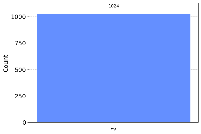
# Replace the NOT gate with a Z gate
q = QuantumRegister(1)
c = ClassicalRegister(1)
qc = QuantumCircuit(q, c)
qc.z(0)
qc.measure(q, c)
print(qc.draw())
simulator = AerSimulator()
results = simulator.run(qc).result().get_counts()
plot_histogram(results)
┌───┐┌─┐
q21: ┤ Z ├┤M├
└───┘└╥┘
c20: 1/══════╩═
0 
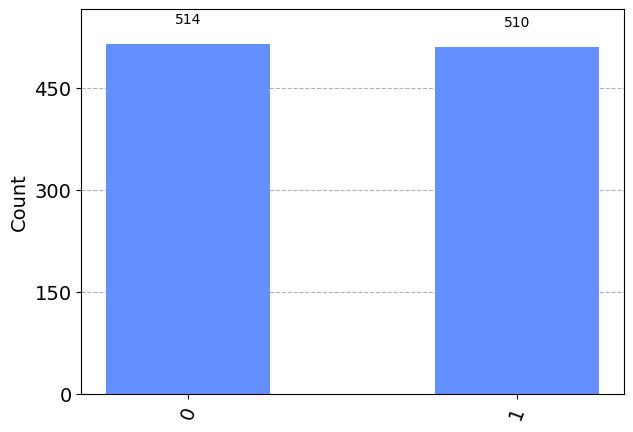
# Replace the Z gate with a Hadamard gate
# Create the plus state
q = QuantumRegister(1)
c = ClassicalRegister(1)
qc = QuantumCircuit(q, c)
qc.h(0)
qc.measure(q, c)
print(qc.draw())
simulator = AerSimulator()
results = simulator.run(qc).result().get_counts()
plot_histogram(results)
┌───┐┌───┐┌─┐
q34: ┤ H ├┤ T ├┤M├
└───┘└───┘└╥┘
c33: 1/═══════════╩═
0 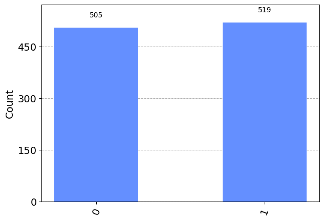
# Chain together a NOT gate and a Hadamard gate
# Creates the minus state
q = QuantumRegister(1)
c = ClassicalRegister(1)
qc = QuantumCircuit(q, c)
qc.x(0)
qc.h(0)
qc.measure(q, c)
print(qc.draw())
simulator = AerSimulator()
results = simulator.run(qc).result().get_counts()
plot_histogram(results)
┌───┐┌───┐┌─┐
q12: ┤ X ├┤ H ├┤M├
└───┘└───┘└╥┘
c11: 1/═══════════╩═
0