Bernstein-Varirani Algorithm and Quantum Fourier Transforms

# Needed to set up the quantum circuit
from qiskit import QuantumCircuit, ClassicalRegister, QuantumRegister
# Needed to simulate running a quantum computer
from qiskit_aer import AerSimulator
# Neded to visualize the results of running a quantum computer
from qiskit.visualization import plot_histogram
# Needed for vectors and stuff
import numpy as np

Bernstein-Vazirani algorithm

The (Absolute Best) Classical Implementation

# This is the "secret string" we want to determine
# Use a vector here to make the dot product easier
s = [1,1,0,1,0,1]

# Get the length of the string and create an array to hold
# the components of s as we recreate them
n = len(s)
reconstructed_s = np.zeros(n)

# Iterate through all indices in the s list
# This iteration runs as many times as there are elements in s
# s is queried n times
for i in range(n):
    # Create a vector of length n that is all zeros and make only
    # the current index 1
    vec = np.zeros(n)
    vec[i] = 1
    # Apply the f(x) function with the vector and the secret string
    f = np.dot(vec,s)%2
    # f is the ith component of s
    reconstructed_s[i] = f

print(s)
print(reconstructed_s)    

[1, 1, 0, 1, 0, 1]
[1. 1. 0. 1. 0. 1.]

Quantum Implementation

The below code is modified from this example provided by IBM through their Qiskit textbook.

Nice but fast video on the topic

# Secret string
# Using a string here to replicate the IBM implementation
s = "110101"
# Get the length of the string
n = len(s)

# Need n+1 qubits. n are mapped to the n classical bits, 
# the last one is used as the oracle/auxillary 
q = QuantumRegister(n+1) 
# Need n classical bits
c = ClassicalRegister(n) 
# creates a quantum circuit that maps the result of a qubit
# to a classical bit
circuit = QuantumCircuit(q, c) 

# Add a not gate the the oracle qubit
circuit.x(n) # the n+1 qubits are indexed 0...n, so the last qubit is index n
circuit.barrier() # just a visual aid for now

# Apply a Hadamard gate to all qubits, this let's you do it in one line
# range(n+1) returns [0,1,2,...,n] in Python. This covers all the qubits
circuit.h(range(n+1)) 
# The first n qubits are in the |+> state 
# and the last qubit is in the |-> state
circuit.barrier() # just a visual aid for now

# enumerate returns the index and value for each element in the string
# Reversed because of the way qiskit displays the results
# Note though that s is only referenced one time
# The number of queries to s is just 1
for i, bit in enumerate(reversed(s)):
    # If the current bit is a one, then add a controlled not 
    # from that bit to the oracle
    if bit == '1': 
        # i is the control qubit, n is the target qubit
        circuit.cx(i, n) 
        # HOWEVER, the oracle qubit is in the |-> state and all of the 
        # other qubits are in the |+> state
        #So phase kickback changes the value of the qubits whose position 
        # corresponds to a 1 in the secret string
circuit.barrier() # just a visual aid for now

# Apply Hadamard gates to all the qubits
# So any remaining in the |+> state become 0 and any that were 
# converted to the |-> state become 1
circuit.h(range(n+1))
circuit.barrier() # just a visual aid for now

# measure the qubits indexed from 0 to n-1 and store them into the 
# classical bits indexed 0 to n-1
# Do not convert the state of the oracle to a classical bit
circuit.measure(range(n), range(n)) 

<qiskit.circuit.instructionset.InstructionSet at 0x11bd5c670>

# The argument makes the circuit look nicer
# There are a few more options as well
# Check the documentation!!
circuit.draw(output='mpl')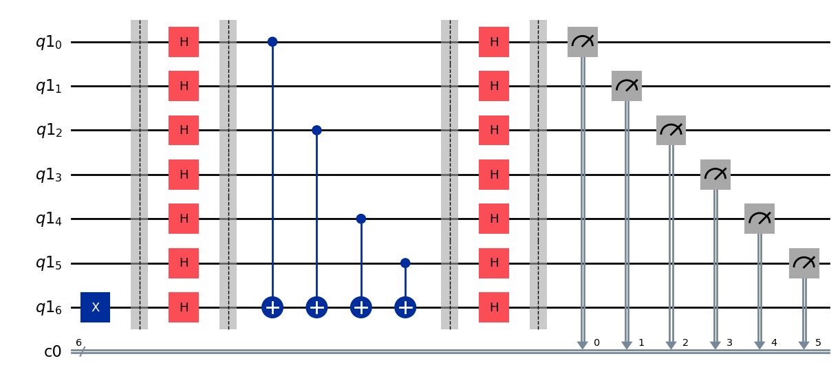

# Simulate the circuit, all results should give us the "secret string"
simulator = AerSimulator()
results = simulator.run(circuit).result().get_counts()
# Print the secret string and then show the histogram of results
print(s)
plot_histogram(results)

110101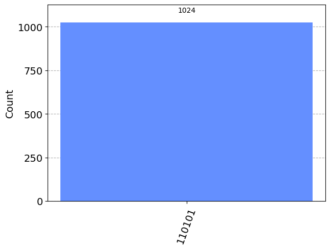

Quantum Fourier Transforms

Classical Implementation

##############################
##      CALCULATE OMEGA     ##
##############################
def calculate_omega (N):
    """
    Calculate the omega constant for the DFT matrix
    Arguments:
        N (int): the size of the DFT matrix
    Returns:
        omega (complex): the omega constant
    """
    omega = np.exp(-2*np.pi*1.0j/N)
    return omega

##############################
##        DFT MATRIX        ##
##############################
def DFT_matrix (N):
    """
    Constructs the DFT matrix at a given size
    Arguments:
        N (int): the size of the DFT matrix
    Returns:
        dft_matrix (a square matrix of complex values): the DFT matrix
    """
    # Placeholder for the DFT matrix. SET THE TYPE TO COMPLEX!!
    dft_matrix = np.ones((N,N), dtype=complex)
    # First column and first row are ones,
    # Only need to change indices 1 through N-1
    # for rows and columns
    omega = calculate_omega(N)
    
    # Iterate over the rows
    for r in range(1,N):
        # Iterate over the columns
        for c in range(1,N):
            # Calculate the matrix element for each opening in the matrix
            dft_matrix[r,c] = (omega)**(r*c)
            
    # Tack on the scaling factor and then return the matrix
    dft_matrix /= np.sqrt(N)
    return dft_matrix
        

# Compute the DFT matrix for two data points
# Look familar?
DFT_matrix(2)

array([[ 0.70710678+0.00000000e+00j,  0.70710678+0.00000000e+00j],
       [ 0.70710678+0.00000000e+00j, -0.70710678-8.65956056e-17j]])

# Compute the DFT matrix for 4 data points
# Round to make the output a bit neater
np.round(DFT_matrix(4),2)

array([[ 0.5+0.j ,  0.5+0.j ,  0.5+0.j ,  0.5+0.j ],
       [ 0.5+0.j ,  0. -0.5j, -0.5-0.j , -0. +0.5j],
       [ 0.5+0.j , -0.5-0.j ,  0.5+0.j , -0.5-0.j ],
       [ 0.5+0.j , -0. +0.5j, -0.5-0.j ,  0. -0.5j]])

##############################
##           DFT            ##
##############################
def dft (x):
    """
    Performs a discrete fourier transform on a given data set and 
    returns the transformed data set
    Arguments:
        x (a Numpy array): the data set to be transformed (should be complex)
    Returns:
        X (a Numpy array): the transformed data set (should be complex and the
            same length as x)
    """
    # Get the length of the data set and then compute the DFT matrix
    N = len(x)
    dft_matrix = DFT_matrix(N)
    
    # Perform DFT by multiplying the data set by the DFT matrix
    X = np.dot(dft_matrix, x)
    
    return X

# Create an example data set, make sure it is complex
x = np.array([1, 2, 3, 4], dtype=complex)  
# Apply DFT to the data set
X = dft(x)

print("Input Data:", x)
print("DFT of the Data:", X)

Input Data: [1.+0.j 2.+0.j 3.+0.j 4.+0.j]
DFT of the Data: [ 5.+0.0000000e+00j -1.+1.0000000e+00j -1.-4.8985872e-16j
 -1.-1.0000000e+00j]

# Compare to the results of using Numpy's discrete fourier transform library
# Note here that fft stands for Fast Fourier Transform, which is an optimized
# version of the discrete fourier transform
X_np = np.fft.fft(x)
print(X_np)

[10.+0.j -2.+2.j -2.+0.j -2.-2.j]

# Note that the above results are not the same as our function because Numpy
# does not apply the normalization constant to the 
X_np = np.fft.fft(x, norm="ortho")
print(X_np)

[ 5.+0.j -1.+1.j -1.+0.j -1.-1.j]

Quantum Implementation

The below code is once again modified from the Qiskit Textbook GitHub.

Quick Detour Through Some New Gates and Qiskit Functionality

# This import let's us visualize the Qiskit qubits as state vectors (bra-ket notation)
from qiskit.quantum_info import Statevector
# This import let's us visualize 
from qiskit.visualization import plot_bloch_multivector

# Create a one qubit circuit with a Hadamard gate and visualize the output
q = QuantumRegister(1)
c = ClassicalRegister(1)
qc = QuantumCircuit(q,c)

qc.h(0)
qc.measure(q,c)
qc.draw(output="mpl")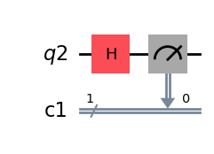

# Remove the measurement (want to keep the superposition to write the output)
qc.remove_final_measurements()  # no measurements allowed
# Get the quantum state that is represented by the circuit
statevector = Statevector(qc)
# Display the state in formatted text
display(statevector.draw(output = 'latex'))

# Convert the qubit to a bloch sphere representation
plot_bloch_multivector(statevector)

\[\frac{\sqrt{2}}{2} |0\rangle+\frac{\sqrt{2}}{2} |1\rangle\]

# Create a three qubit circuit, apply a NOT gate to the first qubit
q = QuantumRegister(3)
c = ClassicalRegister(3)
qc = QuantumCircuit(q,c)
qc.x(0)

# When the state vector is created, the number closest to the angled bracket is
# the first qubit, the number closest to the pipe is the last qubit
qc.remove_final_measurements()  # no measurements allowed
statevector = Statevector(qc)
display(statevector.draw(output = 'latex'))

# The block where prints the diagrams in order, though they are also labelled
# to prevent confusion
plot_bloch_multivector(statevector)

\[ |001\rangle\]

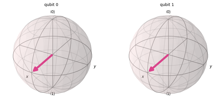
# Note that the state vectors will always be printed with rationalized fractions
# Meaning that here the normalization constants that result from the Hadamard gate are shown
# as sqrt(2)/2 instead of 1/sqrt(2) (these are equivalent)
q = QuantumRegister(2)
c = ClassicalRegister(2)
qc = QuantumCircuit(q,c)
qc.h(0)
qc.x(1)
qc.measure(q,c)

qc.remove_final_measurements()  # no measurements allowed
statevector = Statevector(qc)
display(statevector.draw(output = 'latex'))

plot_bloch_multivector(statevector)

\[\frac{\sqrt{2}}{2} |10\rangle+\frac{\sqrt{2}}{2} |11\rangle\]

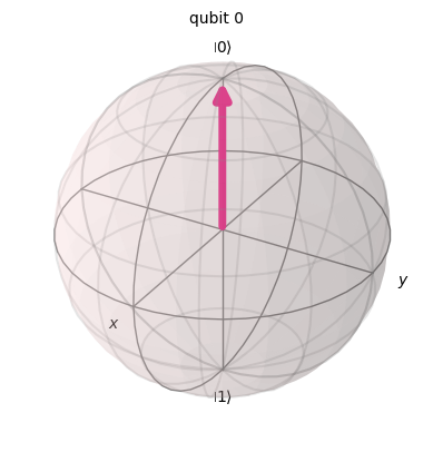
## NEW GATE #1
## The S gate
## The S gate does nothing when applied to the up state

q = QuantumRegister(1)
c = ClassicalRegister(1)
qc = QuantumCircuit(q,c)
qc.s(0)

print(qc.draw())

qc.remove_final_measurements()  # no measurements allowed
statevector = Statevector(qc)
display(statevector.draw(output = 'latex'))

plot_bloch_multivector(statevector)

      ┌───┐
  q5: ┤ S ├
      └───┘
c4: 1/═════
           

\[ |0\rangle\]

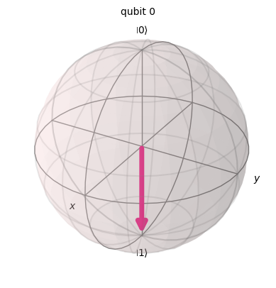
## NEW GATE #1
## The S gate
## The S gate adds a phase factor (constant) of i to the down state
q = QuantumRegister(1)
c = ClassicalRegister(1)
qc = QuantumCircuit(q,c)
qc.x(0)
qc.s(0)

print(qc.draw())

qc.remove_final_measurements()  # no measurements allowed
statevector = Statevector(qc)
display(statevector.draw(output = 'latex'))

plot_bloch_multivector(statevector)

      ┌───┐┌───┐
  q6: ┤ X ├┤ S ├
      └───┘└───┘
c5: 1/══════════
                

\[i |1\rangle\]

## NEW GATE #1
## The Phase gate
## Adds a phase factor if the qubit is down

# Phase angle
theta = np.pi/4

q = QuantumRegister(1)
c = ClassicalRegister(1)
qc = QuantumCircuit(q,c)
qc.x(0)
qc.p(theta, 0)

print(qc.draw())

qc.remove_final_measurements()  # no measurements allowed
statevector = Statevector(qc)
display(statevector.draw(output = 'latex'))

plot_bloch_multivector(statevector)

      ┌───┐┌────────┐
  q7: ┤ X ├┤ P(π/4) ├
      └───┘└────────┘
c6: 1/═══════════════
                     

\[(\frac{\sqrt{2}}{2} + \frac{\sqrt{2} i}{2}) |1\rangle\]

## NEW GATE #3
## The Rz gate
## Rotates the qubit around the z axis for a given number of radians
## Easier to see if we apply a Hadamard gate first to move the qubit
## off the z axis

# Angle of rotation
theta = np.pi/2

q = QuantumRegister(1)
c = ClassicalRegister(1)
qc = QuantumCircuit(q,c)
qc.h(0)
qc.rz(theta,0)

print(qc.draw())

qc.remove_final_measurements()  # no measurements allowed
statevector = Statevector(qc)
display(statevector.draw(output = 'latex'))

plot_bloch_multivector(statevector)

      ┌───┐┌─────────┐
  q8: ┤ H ├┤ Rz(π/2) ├
      └───┘└─────────┘
c7: 1/════════════════
                      

\[(\frac{1}{2} - \frac{i}{2}) |0\rangle+(\frac{1}{2} + \frac{i}{2}) |1\rangle\]

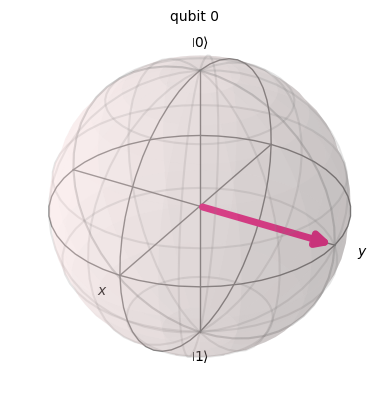
## NEW GATE #4
## The Ry gate
## Rotates the qubit around the y axis for a given number of radians
## What is this equivalent to?

# Angle of rotation
theta = np.pi/2

q = QuantumRegister(1)
c = ClassicalRegister(1)
qc = QuantumCircuit(q,c)
qc.ry(theta,0)

print(qc.draw())

qc.remove_final_measurements()  # no measurements allowed
statevector = Statevector(qc)
display(statevector.draw(output = 'latex'))

plot_bloch_multivector(statevector)

      ┌─────────┐
  q9: ┤ Ry(π/2) ├
      └─────────┘
c8: 1/═══════════
                 

\[\frac{\sqrt{2}}{2} |0\rangle+\frac{\sqrt{2}}{2} |1\rangle\]

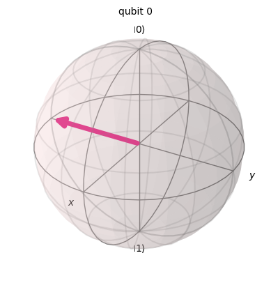
## NEW GATE #5
## The Rx gate
## Rotates the qubit around the x axis for a given number of radians

# Angle of rotation
theta = np.pi/2

q = QuantumRegister(1)
c = ClassicalRegister(1)
qc = QuantumCircuit(q,c)
qc.rx(theta,0)

print(qc.draw())

qc.remove_final_measurements()  # no measurements allowed
statevector = Statevector(qc)
display(statevector.draw(output = 'latex'))

plot_bloch_multivector(statevector)

      ┌─────────┐
 q10: ┤ Rx(π/2) ├
      └─────────┘
c9: 1/═══════════
                 

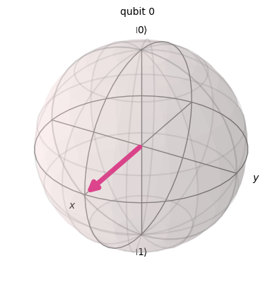
\[\frac{\sqrt{2}}{2} |0\rangle- \frac{\sqrt{2} i}{2} |1\rangle\]

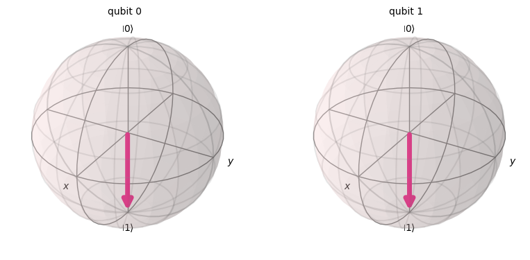
## NEW GATE #6
## The Controlled Phase gate
## Possibly applies a given phase to the target qubit
## This is the main gate for the quantum Fourier algorithm

# Phase angle
theta = np.pi/3

q = QuantumRegister(2)
c = ClassicalRegister(2)
qc = QuantumCircuit(q,c)
# NOT gate for the control qubit to ensure the gate triggers
qc.x(0)
# NOT gate for the target qubit, qubit will only pick up a phase if down
qc.x(1)
# Could also apply a Hadamard gate and then the target qubit will sometimes
# get a phase
#qc.h(1)
# Controlled phase gate
# Arguments are phase angle, control qubit, target qubit
qc.cp(theta,0,1)

print(qc.draw())

qc.remove_final_measurements()  # no measurements allowed
statevector = Statevector(qc)

display(statevector.draw(output = 'latex'))
plot_bloch_multivector(statevector)

       ┌───┐         
q11_0: ┤ X ├─■───────
       ├───┤ │P(π/3) 
q11_1: ┤ X ├─■───────
       └───┘         
c10: 2/══════════════
                     

\[(\frac{1}{2} + \frac{\sqrt{3} i}{2}) |11\rangle\]

## One Qubit Example
pi = np.pi

# Set up a one-qubit circuit
q = QuantumRegister(1)
c = ClassicalRegister(1)
qc = QuantumCircuit(q,c)

# Test different starting conditions
#qc.x(0)
#qc.barrier()

# Apply a Hadamard gate to the qubit and done!
qc.h(0)

# Draw the circuit
print(qc.draw())

# Print the Bloch sphere representation
statevector = Statevector(qc)
plot_bloch_multivector(statevector)

       ┌───┐
  q12: ┤ H ├
       └───┘
c11: 1/═════
            

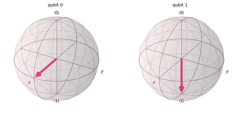
## Two Qubit Example

# Set up a two-qubit circuit
q = QuantumRegister(2)
c = ClassicalRegister(2)
qc = QuantumCircuit(q,c)

# Test different starting conditions
#qc.x(0)
#qc.x(1)

# Apply a Hadamard gate to the highest indexed qubit, so 1
qc.h(1)

# Apply a controlled phase gate from 1 (target) to 0 (control)
# Calculate the angle of rotation
phi = pi/2**(1-0)
qc.cp(phi, 0, 1)

## Apply a Hadamard gate to the next highest indexed qubit, so 0
qc.h(0)

## Done with Hadamard and CPhase gate, now just swap the qubits
qc.swap(0,1)

# Draw the circuit
print(qc.draw())

# Print the Bloch sphere representation
statevector = Statevector(qc)
plot_bloch_multivector(statevector)

# Print the Bloch sphere representation
statevector = Statevector(qc)
plot_bloch_multivector(statevector)

                     ┌───┐   
q13_0: ──────■───────┤ H ├─X─
       ┌───┐ │P(π/2) └───┘ │ 
q13_1: ┤ H ├─■─────────────X─
       └───┘                 
c12: 2/══════════════════════
                             

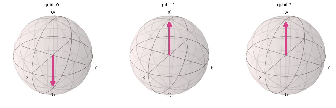
## Three Qubit Example

# Set up a two-qubit circuit
q = QuantumRegister(3)
c = ClassicalRegister(3)
qc = QuantumCircuit(q,c)

# Test different starting conditions
#qc.x(0)
#qc.x(1)
#qc.x(2)
#qc.barrier()

# Apply a Hadamard gate to the highest indexed qubit, so 2
qc.h(2)

# Apply a controlled phase gate from 2 (target) to 1 (control)
# Calculate the angle of rotation
phi = pi/2**(2-1)
qc.cp(phi, 1, 2)

# Apply a controlled phase gate from 2 (target) to 0 (control)
# Calculate the angle of rotation
phi = pi/2**(2-0)
qc.cp(phi, 0, 2)

## Apply a Hadamard gate to the next highest indexed qubit, so 1
qc.h(1)

# Apply a controlled phase gate from 1 (target) to 0 (control)
# Calculate the angle of rotation
phi = pi/2**(1-0)
qc.cp(phi, 0, 1)

## Apply a Hadamard gate to the next highest indexed qubit, so 0
qc.h(0)

## Done with Hadamard and CPhase gate, now just swap the qubits
## For three qubits it is sufficient to just swap the order of 0 and 2
qc.swap(0,2)

# Draw the circuit
print(qc.draw())

# Print the Bloch sphere representation
statevector = Statevector(qc)
plot_bloch_multivector(statevector)

                                            ┌───┐   
q16_0: ───────────────■─────────────■───────┤ H ├─X─
                      │       ┌───┐ │P(π/2) └───┘ │ 
q16_1: ──────■────────┼───────┤ H ├─■─────────────┼─
       ┌───┐ │P(π/2)  │P(π/4) └───┘               │ 
q16_2: ┤ H ├─■────────■───────────────────────────X─
       └───┘                                        
c15: 3/═════════════════════════════════════════════
                                                    

Generalized Code

def qft_rotations(circuit, n):
    """
        Performs qft on the first n qubits in circuit (without swaps)
        Inputs:
            circuit is the qiskit circuit
            n is the number of qubits in the circuit
        Returns
            circuit after adding Hadamard gates and controlled phase gates to perform
                the qft
    """
    # Break condition
    if n == 0:
        return circuit
        
    # Subtract 1 because the highest indexed qubit is one less than the total number of qubits
    n -= 1
    # Hadamard to the highest indexed qubit
    circuit.h(n)
    # Controlled phase gate with the qubit at n (the highest ordered) being the target and every
    # lower indexed qubit being the control in order
    for qubit in range(n):
        phi = pi/2**(n-qubit)
        circuit.cp(phi, qubit, n)
    
    # Recursion time!
    # Recall the function with the same circuit, but n is one less than it was originally
    # The next run-through will ignore the highest indexed qubit in this run-through
    qft_rotations(circuit, n)

def swap_qubits(circuit, n):
    """
        Performs swaps the locations of all qubits
        Inputs:
            circuit is the qiskit circuit
            n is the number of qubits in the circuit
        Returns
            circuit after swapping all qubits
    """
    # Int in range function because range requires an integer
    for qubit in range(int(n/2)):
        # swap the position of a low-indexed qubit and the qubit
        # that is the same distance from the highest ordered qubit
        circuit.swap(qubit, n-qubit-1)
    return circuit

def qft(circuit, n):
    """
        Performs QFT on a qiskit circuit by adding the correct gates to the circuit and then
        swapping the order of the qubits
        Inputs:
            circuit is the qiskit circuit
            n is the number of qubits in the circuit
        Returns:
            circuit is the qiskit circuit after the qft gates are applied            
    """
    qft_rotations(circuit, n)
    swap_qubits(circuit, n)
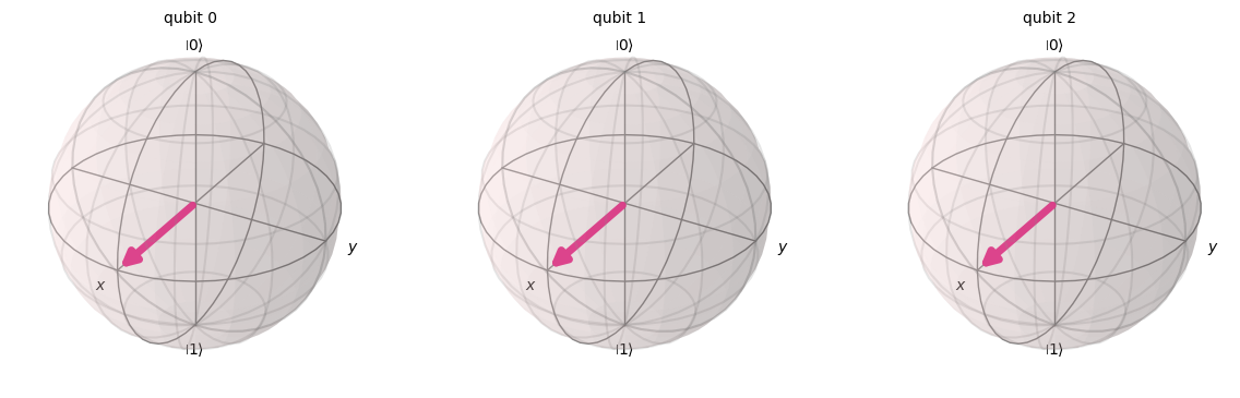
    return circuit

## Example!

qc = QuantumCircuit(3)

# Encode the state 5
qc.x(0)
qc.x(2)
print(qc.draw())
qc.remove_final_measurements()  # no measurements allowed
statevector = Statevector(qc)
plot_bloch_multivector(statevector)

     ┌───┐
q_0: ┤ X ├
     └───┘
q_1: ─────
     ┌───┐
q_2: ┤ X ├
     └───┘

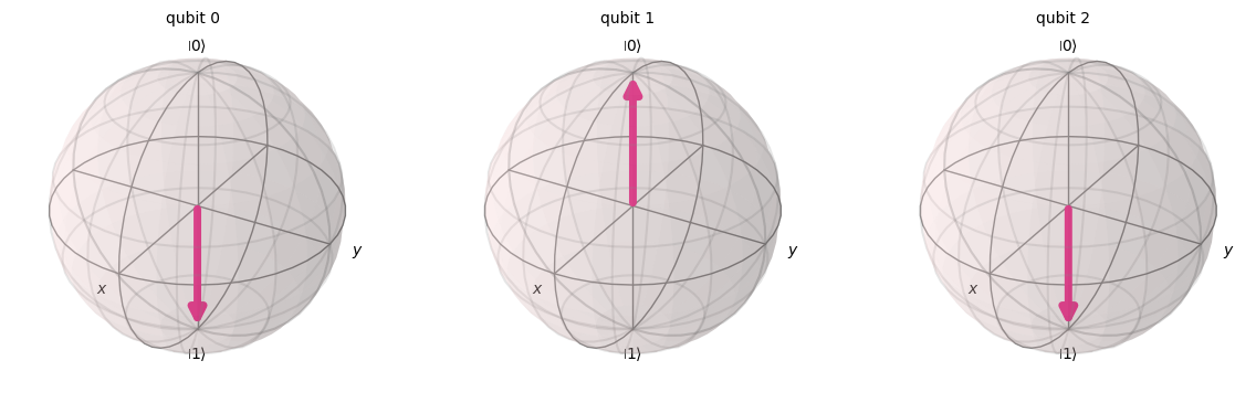
qft(qc,3)
qc.draw()

     ┌───┐                                     ┌───┐   
q_0: ┤ X ├──────■──────────────────────■───────┤ H ├─X─
     └───┘      │                ┌───┐ │P(π/2) └───┘ │ 
q_1: ───────────┼────────■───────┤ H ├─■─────────────┼─
     ┌───┐┌───┐ │P(π/4)  │P(π/2) └───┘               │ 
q_2: ┤ X ├┤ H ├─■────────■───────────────────────────X─
     └───┘└───┘                                        

# Bloch sphere diagram
qc.remove_final_measurements()  # no measurements allowed
statevector = Statevector(qc)
plot_bloch_multivector(statevector)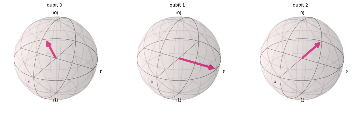

## Important Note: the QFT creates a superposition of many possible states
## The phase factors added by the Hadamard gates and controlled phase gates will be important 
## in applications
## Note that all possible three qubit states are represented here
display(statevector.draw(output = 'latex'))

\[\frac{\sqrt{2}}{4} |000\rangle+(- \frac{1}{4} - \frac{i}{4}) |001\rangle+\frac{\sqrt{2} i}{4} |010\rangle+(\frac{1}{4} - \frac{i}{4}) |011\rangle- \frac{\sqrt{2}}{4} |100\rangle+(\frac{1}{4} + \frac{i}{4}) |101\rangle- \frac{\sqrt{2} i}{4} |110\rangle+(- \frac{1}{4} + \frac{i}{4}) |111\rangle\]

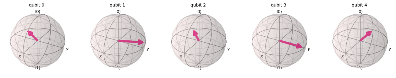
n = 5
qc = QuantumCircuit(n)
qc.x(0)
#qc.x(1)
qc.x(2)
#qc.x(3)
qc.x(4)
qft(qc,n)
print(qc.draw())
qc.remove_final_measurements()  # no measurements allowed
statevector = Statevector(qc)
plot_bloch_multivector(statevector)

     ┌───┐                                                                 »
q_0: ┤ X ├──────■─────────────────────────────────────────■────────────────»
     └───┘      │                                         │                »
q_1: ───────────┼─────────■───────────────────────────────┼────────■───────»
     ┌───┐      │         │                               │        │       »
q_2: ┤ X ├──────┼─────────┼────────■──────────────────────┼────────┼───────»
     └───┘      │         │        │                ┌───┐ │P(π/8)  │P(π/4) »
q_3: ───────────┼─────────┼────────┼────────■───────┤ H ├─■────────■───────»
     ┌───┐┌───┐ │P(π/16)  │P(π/8)  │P(π/4)  │P(π/2) └───┘                  »
q_4: ┤ X ├┤ H ├─■─────────■────────■────────■──────────────────────────────»
     └───┘└───┘                                                            »
«                                                   ┌───┐   
«q_0: ───────────────■──────────────────────■───────┤ H ├─X─
«                    │                ┌───┐ │P(π/2) └───┘ │ 
«q_1: ───────────────┼────────■───────┤ H ├─■─────────X───┼─
«              ┌───┐ │P(π/4)  │P(π/2) └───┘           │   │ 
«q_2: ─■───────┤ H ├─■────────■───────────────────────┼───┼─
«      │P(π/2) └───┘                                  │   │ 
«q_3: ─■──────────────────────────────────────────────X───┼─
«                                                         │ 
«q_4: ────────────────────────────────────────────────────X─
«