More Quantum Fourier Transforms, Quantum Phase Estimation, and Quantum Parallelism

A Few Final QFT Topics

# Needed to set up the quantum circuit
from qiskit import QuantumCircuit, ClassicalRegister, QuantumRegister
# Needed to simulate running a quantum computer
from qiskit_aer import AerSimulator
# Neded to visualize the results of running a quantum computer
from qiskit.visualization import plot_histogram
# Needed for vectors and stuff
import numpy as np
# This import let's us visualize the Qiskit qubits as state vectors (bra-ket notation)
from qiskit.quantum_info import Statevector
# This import let's us visualize 
from qiskit.visualization import plot_bloch_multivector

def qft_rotations(circuit, n):
    """
        Performs qft on the first n qubits in circuit (without swaps)
        Inputs:
            circuit is the qiskit circuit
            n is the number of qubits in the circuit
        Returns
            circuit after adding Hadamard gates and controlled phase gates to perform
                the qft
    """
    # Break condition
    if n == 0:
        return circuit
        
    # Define pi
    pi = np.pi
    # Subtract 1 because the highest indexed qubit is one less than the total number of qubits
    n -= 1
    # Hadamard to the highest indexed qubit
    circuit.h(n)
    # Controlled phase gate with the qubit at n (the highest ordered) being the target and every
    # lower indexed qubit being the control in order
    for qubit in range(n):
        phi = pi/2**(n-qubit)
        circuit.cp(phi, qubit, n)
    
    # Recursion time!
    # Recall the function with the same circuit, but n is one less than it was originally
    # The next run-through will ignore the highest indexed qubit in this run-through
    qft_rotations(circuit, n)

def swap_qubits(circuit, n):
    """
        Performs swaps the locations of all qubits
        Inputs:
            circuit is the qiskit circuit
            n is the number of qubits in the circuit
        Returns
            circuit after swapping all qubits
    """
    # Int in range function because range requires an integer
    for qubit in range(int(n/2)):
        # swap the position of a low-indexed qubit and the qubit
        # that is the same distance from the highest ordered qubit
        circuit.swap(qubit, n-qubit-1)
    return circuit

def qft(circuit, n):
    """
        Performs QFT on a qiskit circuit by adding the correct gates to the circuit and then
        swapping the order of the qubits
        Inputs:
            circuit is the qiskit circuit
            n is the number of qubits in the circuit
        Returns:
            circuit is the qiskit circuit after the qft gates are applied            
    """
    qft_rotations(circuit, n)
    swap_qubits(circuit, n)
    return circuit

## Example!

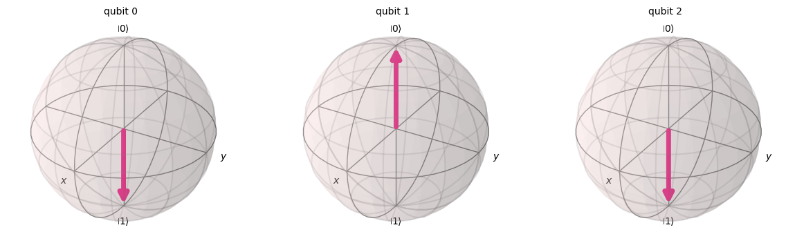
q = QuantumRegister(3)
c = ClassicalRegister(3)
qc = QuantumCircuit(q,c)

# Encode the state 5
qc.x(0)
qc.x(2)

print(qc.draw())

statevector = Statevector(qc)
plot_bloch_multivector(statevector)

      ┌───┐
q1_0: ┤ X ├
      └───┘
q1_1: ─────
      ┌───┐
q1_2: ┤ X ├
      └───┘
c0: 3/═════
           

qft(qc,3)
qc.draw()

      ┌───┐                                     ┌───┐   
q1_0: ┤ X ├──────■──────────────────────■───────┤ H ├─X─
      └───┘      │                ┌───┐ │P(π/2) └───┘ │ 
q1_1: ───────────┼────────■───────┤ H ├─■─────────────┼─
      ┌───┐┌───┐ │P(π/4)  │P(π/2) └───┘               │ 
q1_2: ┤ X ├┤ H ├─■────────■───────────────────────────X─
      └───┘└───┘                                        
c0: 3/══════════════════════════════════════════════════
                                                        

# Bloch sphere diagram
qc.remove_final_measurements()  # no measurements allowed
statevector = Statevector(qc)
plot_bloch_multivector(statevector)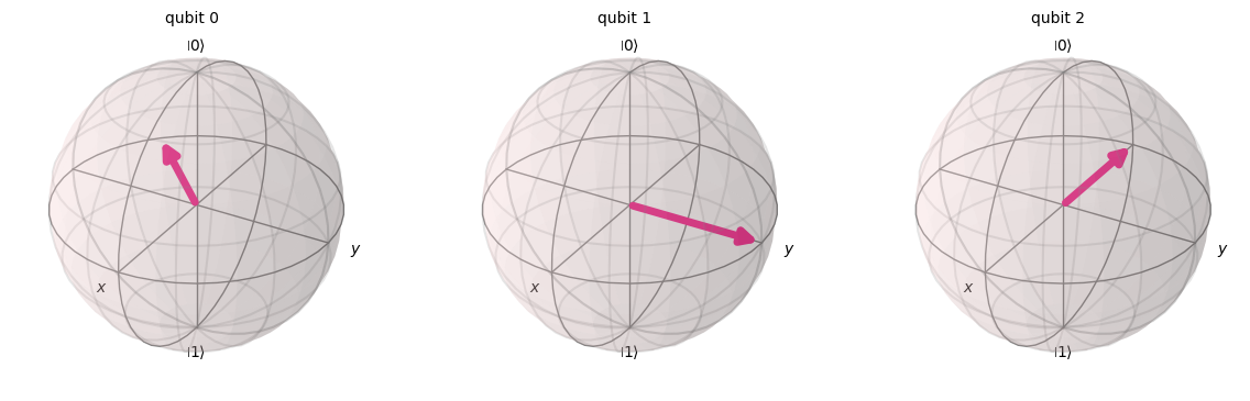

## Can also perform QFT using the built-in function
from qiskit.circuit.library import QFT

# Create a 3-qubit Quantum Circuit
q = QuantumRegister(3)
c = ClassicalRegister(3)
qc = QuantumCircuit(q,c)

# Encode the binary 5 to compare to out results
qc.x(0)
qc.x(2)

# Apply a QFT on the qubits
qft_circuit = QFT(num_qubits=3)
qc.append(qft_circuit.to_instruction(), range(3))

# Draw the circuit
qc.draw(output='mpl')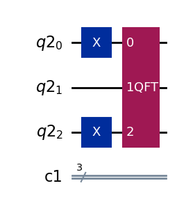

# Same Results!
statevector = Statevector(qc)
plot_bloch_multivector(statevector)

# Apply an Inverse QFT on the qubits of the same circuit
qft_circuit = QFT(num_qubits=3, inverse=True)
qc.append(qft_circuit.to_instruction(), range(3))

# Draw the circuit
qc.draw(output='mpl')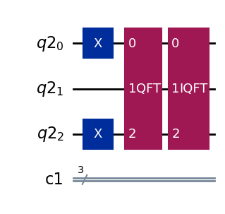

# The result should be a binary 5!
statevector = Statevector(qc)
plot_bloch_multivector(statevector)

Quantum Phase Estimation

## Let's start off easy. Our controlled U gate is just the 
# controlled phase gate with some specific angle. 
phi = 2*np.pi/3

## Let's start by measuring the precision of the eigenvalue to three decimal places, 
## so we need 4 qubits mapping to three classical bits (we do not measure 
## the eigenvector qubit)

q = QuantumRegister(4)
c = ClassicalRegister(3)
qc = QuantumCircuit(q,c)

## First we need to make sure the last qubit is in an eigenstate of the U gate. 
## The up and down states are both possible eigenvectors but up is trivial 
## (has an eigenvalue of 1) so let's go with down

qc.x(3)
qc.barrier()

## Now Hadamard gates for the other qubits
qc.h(0)
qc.h(1)
qc.h(2)
qc.barrier()

## Controlled U gate from eigenvector qubit (target) to highest indexed H gated qubit
qc.cp(phi, 2, 3)
qc.barrier()

## Now two controlled U gates from eigenvector qubit (target) 
## to second highest indexed H gated qubit
qc.cp(phi, 1, 3)
qc.cp(phi, 1, 3)
qc.barrier()

## Finally four controleld U gates from eigenvector qubit target) 
## to lowest index H gated qubit
qc.cp(phi, 0, 3)
qc.cp(phi, 0, 3)
qc.cp(phi, 0, 3)
qc.cp(phi, 0, 3)
qc.barrier()

## Finally the IQFT but only on the first three qubits
qc = qc.compose(QFT(3, inverse=True), [0,1,2])
qc.barrier()

# Measure of course!
for n in range(3):
    qc.measure(n,n)
qc.barrier()    


qc.draw(output="mpl")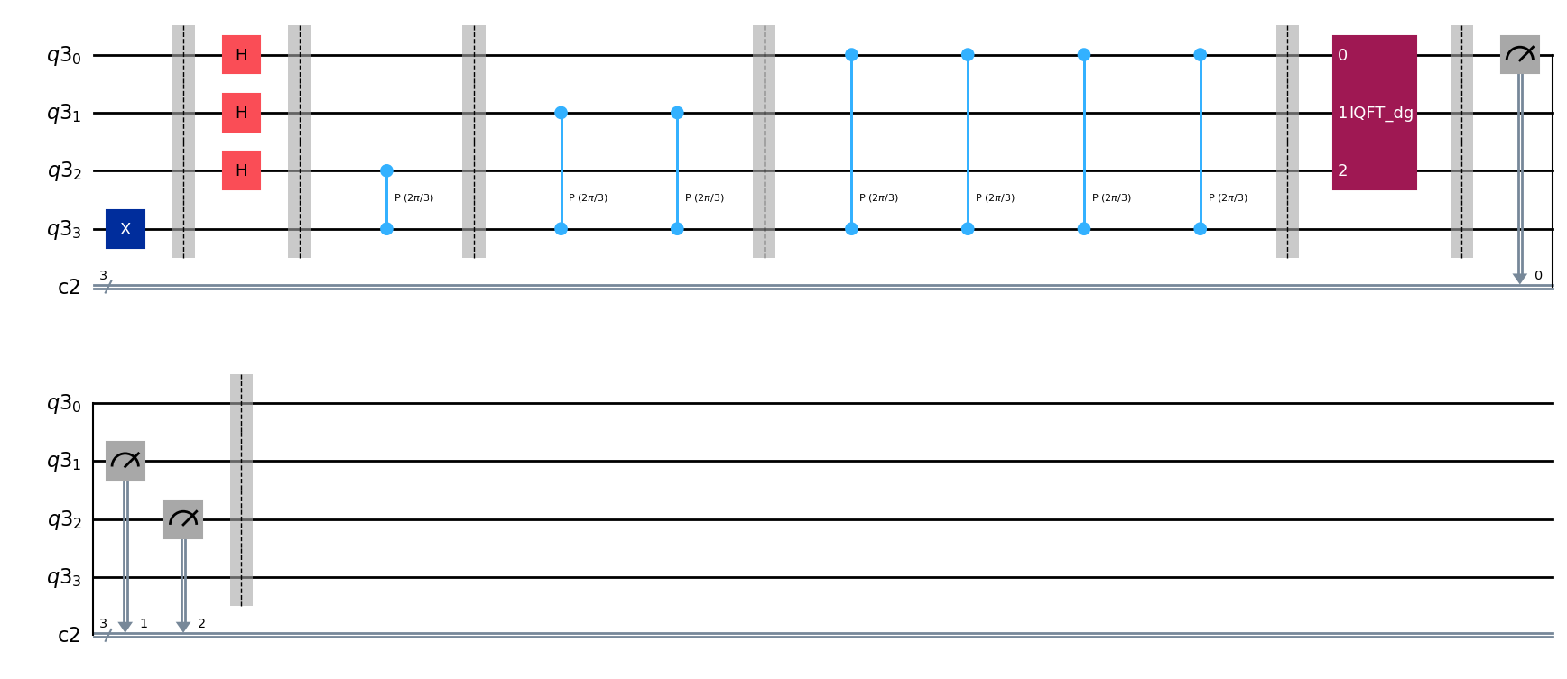

# importing Qiskit transpile
from qiskit import transpile


simulator = AerSimulator()
# Number of times to simulate
shots = 2048
# Need to transpile since using the IQFT "black box" function
# transpile converts the black box into its invividual gates
t_qpe = transpile(qc, simulator)

results = simulator.run(t_qpe, shots=shots).result()
answer = results.get_counts()
plot_histogram(answer)

/Users/butlerju/Library/Python/3.9/lib/python/site-packages/urllib3/__init__.py:35: NotOpenSSLWarning: urllib3 v2 only supports OpenSSL 1.1.1+, currently the 'ssl' module is compiled with 'LibreSSL 2.8.3'. See: https://github.com/urllib3/urllib3/issues/3020
  warnings.warn(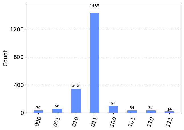

## First example where there is more than one possible answer due 
## to the Hadamard gates and quantum parallelism, but most likely 
## answer is the one with the higest number of results

print("Known Angle:", phi)
print("Most Likely Result:", 2*np.pi*(0/2+1/4+1/8))
print("Also Likely:", 2*np.pi*(0/2+1/4+0/8))

## To get better results, add more counting qubits!

Known Angle: 2.0943951023931953
Most Likely Result: 2.356194490192345
Also Likely: 1.5707963267948966

## WARNING: This starts to really chug above 10 qubits 
## (remember this is a simulated quantum computer,
# not a real one)

## Let's start off easy. Our controlled U gate is just the controlled 
## phase gate with some specific angle. 
phi = np.pi/3

## Make it general now to work with any number of qubits
counting_qubits = 5

# Need one more qubit than bit
q = QuantumRegister(counting_qubits + 1)
c = ClassicalRegister(counting_qubits)
qc = QuantumCircuit(q,c)

## First we need to make sure the last qubit is in an eigenstate of the U gate. 
## The up and down states are both possible eigenvectors but up is trivial 
## (has an eigenvalue of 1) so let's go with down
qc.x(counting_qubits)
qc.barrier()

# Apply H-Gates to counting qubits:
for qubit in range(counting_qubits):
    qc.h(qubit)
qc.barrier()
    
# Do the controlled-U operations:
repetitions = 1
for control in range(counting_qubits):
    for i in range(repetitions):
        qc.cp(phi, control, counting_qubits)
    qc.barrier()
    repetitions *= 2

# Do the inverse QFT:
qc = qc.compose(QFT(counting_qubits, inverse=True), range(counting_qubits))
qc.barrier()

# Measure of course!
for n in range(counting_qubits):
   qc.measure(n,n)

qc.draw()

             ░ ┌───┐ ░           ░                    ░                   »
q10_0: ──────░─┤ H ├─░──■────────░────────────────────░───────────────────»
             ░ ├───┤ ░  │        ░                    ░                   »
q10_1: ──────░─┤ H ├─░──┼────────░──■────────■────────░───────────────────»
             ░ ├───┤ ░  │        ░  │        │        ░                   »
q10_2: ──────░─┤ H ├─░──┼────────░──┼────────┼────────░──■────────■───────»
             ░ ├───┤ ░  │        ░  │        │        ░  │        │       »
q10_3: ──────░─┤ H ├─░──┼────────░──┼────────┼────────░──┼────────┼───────»
             ░ ├───┤ ░  │        ░  │        │        ░  │        │       »
q10_4: ──────░─┤ H ├─░──┼────────░──┼────────┼────────░──┼────────┼───────»
       ┌───┐ ░ └───┘ ░  │P(π/3)  ░  │P(π/3)  │P(π/3)  ░  │P(π/3)  │P(π/3) »
q10_5: ┤ X ├─░───────░──■────────░──■────────■────────░──■────────■───────»
       └───┘ ░       ░           ░                    ░                   »
 c3: 5/═══════════════════════════════════════════════════════════════════»
                                                                          »
«                          ░                                              »
«q10_0: ───────────────────░──────────────────────────────────────────────»
«                          ░                                              »
«q10_1: ───────────────────░──────────────────────────────────────────────»
«                          ░                                              »
«q10_2: ─■────────■────────░──────────────────────────────────────────────»
«        │        │        ░                                              »
«q10_3: ─┼────────┼────────░──■────────■────────■────────■────────■───────»
«        │        │        ░  │        │        │        │        │       »
«q10_4: ─┼────────┼────────░──┼────────┼────────┼────────┼────────┼───────»
«        │P(π/3)  │P(π/3)  ░  │P(π/3)  │P(π/3)  │P(π/3)  │P(π/3)  │P(π/3) »
«q10_5: ─■────────■────────░──■────────■────────■────────■────────■───────»
«                          ░                                              »
« c3: 5/══════════════════════════════════════════════════════════════════»
«                                                                         »
«                                   ░                                     »
«q10_0: ────────────────────────────░─────────────────────────────────────»
«                                   ░                                     »
«q10_1: ────────────────────────────░─────────────────────────────────────»
«                                   ░                                     »
«q10_2: ────────────────────────────░─────────────────────────────────────»
«                                   ░                                     »
«q10_3: ─■────────■────────■────────░─────────────────────────────────────»
«        │        │        │        ░                                     »
«q10_4: ─┼────────┼────────┼────────░──■────────■────────■────────■───────»
«        │P(π/3)  │P(π/3)  │P(π/3)  ░  │P(π/3)  │P(π/3)  │P(π/3)  │P(π/3) »
«q10_5: ─■────────■────────■────────░──■────────■────────■────────■───────»
«                                   ░                                     »
« c3: 5/══════════════════════════════════════════════════════════════════»
«                                                                         »
«                                                                      »
«q10_0: ───────────────────────────────────────────────────────────────»
«                                                                      »
«q10_1: ───────────────────────────────────────────────────────────────»
«                                                                      »
«q10_2: ───────────────────────────────────────────────────────────────»
«                                                                      »
«q10_3: ───────────────────────────────────────────────────────────────»
«                                                                      »
«q10_4: ─■────────■────────■────────■────────■────────■────────■───────»
«        │P(π/3)  │P(π/3)  │P(π/3)  │P(π/3)  │P(π/3)  │P(π/3)  │P(π/3) »
«q10_5: ─■────────■────────■────────■────────■────────■────────■───────»
«                                                                      »
« c3: 5/═══════════════════════════════════════════════════════════════»
«                                                                      »
«                                                     ░ ┌──────────┐ ░ ┌─┐   »
«q10_0: ──────────────────────────────────────────────░─┤0         ├─░─┤M├───»
«                                                     ░ │          │ ░ └╥┘┌─┐»
«q10_1: ──────────────────────────────────────────────░─┤1         ├─░──╫─┤M├»
«                                                     ░ │          │ ░  ║ └╥┘»
«q10_2: ──────────────────────────────────────────────░─┤2 IQFT_dg ├─░──╫──╫─»
«                                                     ░ │          │ ░  ║  ║ »
«q10_3: ──────────────────────────────────────────────░─┤3         ├─░──╫──╫─»
«                                                     ░ │          │ ░  ║  ║ »
«q10_4: ─■────────■────────■────────■────────■────────░─┤4         ├─░──╫──╫─»
«        │P(π/3)  │P(π/3)  │P(π/3)  │P(π/3)  │P(π/3)  ░ └──────────┘ ░  ║  ║ »
«q10_5: ─■────────■────────■────────■────────■────────░──────────────░──╫──╫─»
«                                                     ░              ░  ║  ║ »
« c3: 5/════════════════════════════════════════════════════════════════╩══╩═»
«                                                                       0  1 »
«                
«q10_0: ─────────
«                
«q10_1: ─────────
«       ┌─┐      
«q10_2: ┤M├──────
«       └╥┘┌─┐   
«q10_3: ─╫─┤M├───
«        ║ └╥┘┌─┐
«q10_4: ─╫──╫─┤M├
«        ║  ║ └╥┘
«q10_5: ─╫──╫──╫─
«        ║  ║  ║ 
« c3: 5/═╩══╩══╩═
«        2  3  4 

# Run the simulation
simulator = AerSimulator()
shots = 2048
t_qpe = transpile(qc, simulator)
results = simulator.run(t_qpe, shots=shots).result()
answer = results.get_counts()

# Sort the returned dictionary in order of counts of each result
sorted_answer = sorted(answer, key=answer.get, reverse=True)

# Write a little function to convert the output of the quantum circuit
# to an angle

##############################
##     CONVERT TO ANGLE     ##
##############################
def convert_to_angle(b):
    """
        Converts a binary string to an angle using the quantum phase estimation
        algorithm
        Inputs:
            b (a binary string)
        Returns:
            angle (a float): the corresponding angle
    """
    sum = 0
    for i in range(len(b)):
        sum += int(b[i])/2**(i+1)
    angle = sum*2*np.pi
    return angle

## NOTE: Since we are using the controlled phase gate, we only need to look at the angle
## In general, the eigenvalue is e^{i\theta}, not just the angle

print("Known Angle:", phi)
print()
print("Most Likely Angle:", convert_to_angle(sorted_answer[0]))
print("Probability:", answer[sorted_answer[0]]/shots)
print()
print("Second Most Likely Angle:", convert_to_angle(sorted_answer[1]))
print("Probability:", answer[sorted_answer[1]]/shots)
print()
print("Third Most Likely Angle:", convert_to_angle(sorted_answer[2]))
print("Probability:", answer[sorted_answer[2]]/shots)
print()

Known Angle: 1.0471975511965976

Most Likely Angle: 0.9817477042468103
Probability: 0.6904296875

Second Most Likely Angle: 1.1780972450961724
Probability: 0.15771484375

Third Most Likely Angle: 0.7853981633974483
Probability: 0.04443359375