Grover’s Search Algorithm

# Non-qiskit imports
import math
import numpy as np
import matplotlib.pyplot as plt

# Imports from Qiskit
from qiskit import QuantumCircuit, QuantumRegister, ClassicalRegister
from qiskit.circuit.library import GroverOperator, MCMT, ZGate, XGate
from qiskit.visualization import  plot_histogram
from qiskit.quantum_info import Statevector

# Imports from Qiskit Simulator
from qiskit_aer import AerSimulator
from qiskit import transpile

Clasical Search for Unsorted Data

# Create a graph which shows the difference between O(N) and O(sqrt(N)) 
# compitational efficiency which searching through large lists

# Create a variable for the size of the list, holding data from 10^1 to
# 10^10. There are 50 total points
x = np.logspace(1, 10, 50)

# Classical scaling for an unsorted search algorithm is O(N)
classical = x
# Quantum scaling for an unsorted search algorithm is O(sqrt(N))
quantum = np.sqrt(x)

# Plot the computational efficiencies, format the graph, add labels and a legend
plt.plot(x,classical, linewidth=2, color="darkred", label="Classical")
plt.plot(x,quantum, linewidth=2, color="darkblue", linestyle="--", label="Quantum")
plt.xticks(fontfamily="serif")
plt.yticks(fontfamily="serif")
plt.xlabel("Number of Elements in List", fontsize=14, fontfamily="serif")
plt.ylabel("Computational Efficiency", fontsize=14, fontfamily="serif")
plt.legend(prop={'family':"serif", 'size':12})

# Save the image
plt.savefig("grover_comp_eff.png", dpi=1000)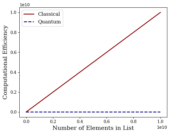

##############################
##  LINEAR SEARCH VERSION 1 ##
##############################
def linear_search_version_1 (my_list, element):
    """
        Brute force search of an element in a list. The list
        does not have to be sorted
        Inputs:
            my_list (a list)
            element (int/float/string): the element to be found in the list  
        Returns
            i (an int): returns the index where the element was found, returns
                -1 if the element was not found            
    """
    length = len(my_list)
    for i in range(length):
        if my_list[i] == element:
            return i
    return -1

##############################
##     MAKE SEARCH LIST     ##
##############################
def make_search_list (length, max_val, ensured_val):
    """
        Creates a list of integers of a given length between zero and one less than
        the maximum value passed. Then, it ensures that a given value is randomly placed
        in the list
        Inputs:
            length (an int): the length of the list
            max_val (an int): the maximum value (+1) to include in the list of integers
            ensured_val (int/float): the value to make sure is in the list
        Returns:
            my_list(a numpy array): a list of integers with the wanted element randomly placed
                in the list
    """
    my_list = np.random.randint(0, max_val, length)
    random_index = np.random.randint(length)
    my_list[random_index] = ensured_val
    return my_list

## Create unsorted list to search through
n = int(1e5)
my_list = make_search_list(n, n, 3) 

print((my_list==3).sum()) # Print the number of occurrences of the wanted element

2

%%time
# Perform a linea search on the list
print(linear_search_version_1(my_list, 3)) # Does not have to be sorted for linear search

5371
CPU times: user 3.58 ms, sys: 171 µs, total: 3.76 ms
Wall time: 1.34 ms

##############################
##  LINEAR SEARCH VERSION 2 ##
##############################
def linear_search_version_2 (my_list, element):
    """
        Brute force search of an element in a list. The list
        does not have to be sorted. Return a list where the element
        is 1 if it is in the same location as the wanted element, 0 if not
        Inputs:
            my_list (a list)
            element (int/float/string): the element to be found in the list  
        Returns:
            results (a list): if the wanted element is found at a given index, then
                the element at the same index in results is 1. Otherwise, results has
                a zero at the element
                   
    """
    length = len(my_list)
    results = np.zeros(length)
    for i in range(length):
        if my_list[i] == element:
            results[i] = 1
    return results

## Create a test list
n = int(1e5)
my_list = make_search_list(n, n, 3) 

print((my_list==3).sum()) # Print the number of occurrences of the wanted element

1

%%time
# Plot the results
results = linear_search_version_2(my_list, 3) # Does not have to be sorted for linear search
plt.plot(range(n), results)

CPU times: user 115 ms, sys: 6.06 ms, total: 121 ms
Wall time: 50 ms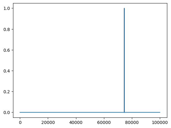

Two Qubit Example

This code is modified from the archived Qiskit textbook. The original algorithm, as proposed by Grover, can be found in this paper.

# Define a two qubit quantum circuit
n = 2
q = QuantumRegister(n)
c = ClassicalRegister(n)
grover_circuit = QuantumCircuit(q,c)

# Add Hadamard gates to both bits
grover_circuit.h(range(n))
grover_circuit.barrier()

# The oracle is simply a controlled Z gate as
# this will add a phase of pi (phase = e^(i\pi))
# to the wanted state only (wanted state is |11>)
grover_circuit.cz(0,1) # Oracle
grover_circuit.barrier()

# Now add the amplification operator for a two
# qubit system
# Hadamard gates to all qubits
grover_circuit.h([0,1])
# NOT gates to all qubits
grover_circuit.x([0,1])
# Controlled Z where the last qubit is the target,
# the first qubit is the control
grover_circuit.cz(0,1)
# NOT gates to all qubits
grover_circuit.x([0,1])
# Hadamard gates to all qubits
grover_circuit.h([0,1])
grover_circuit.barrier()

# Measure the state of the qubits
grover_circuit.measure(range(n), range(n))

# Draw the circuit
grover_circuit.draw(output="mpl")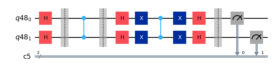

# Simulate the circuit with no need to transpile since there are no combination
# gates, the only result should be the desired state
simulator = AerSimulator()
results = simulator.run(grover_circuit).result().get_counts()
plot_histogram(results)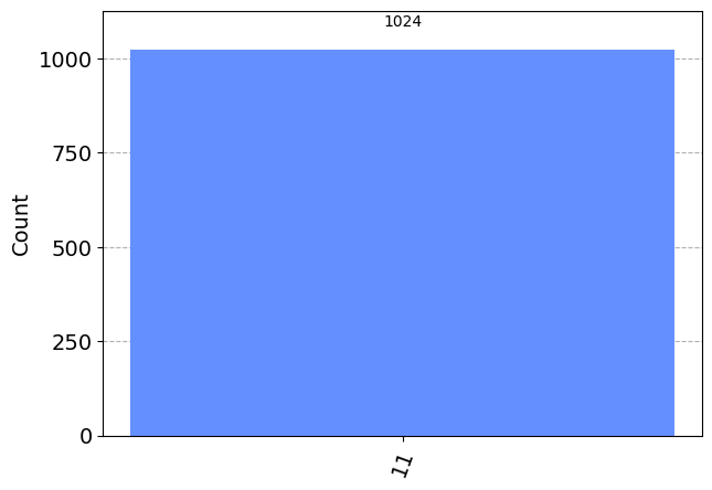

General Case

This code is modified from this project created by Qiskit. Additional code is modified from the archived Qiskit textbook.

Note that Qiskit has many built-in Grover’s algorithm functions. Here we will be creating our own oracle but will use Qiskit’s amplification code.

All Individual Gates

Here we will build the Grover’s algorithm oracle and amplification circuits using base gates

def grover_oracle(qc, num_qubits, marked_states):
    """
        Create a Grover's algorithm oracle for the general case of finding some number
        of marked strings from a list of all possible binary strings fo a given length.
        Inputs:
            qc (a qiskit circuit): The qiskit circuit to add the oracle to
            num_qubits (an int): The number of qubits in the circuit
            marked_states (a list): the states to mark for the grover's Algorithm to find
    """
    # Create a barrier to mark the start of the algorithm
    qc.barrier()
    
    # Mark each target state in the input list
    for target in marked_states:
        
        # Flip target bit-string to match Qiskit bit-ordering
        rev_target = target[::-1]
        
        # Find the indices of all the '0' elements in bit-string
        # NOT gate will be placed at these values
        # NOTE ERRORS OUT IF NO 0 STATES FOUND IN STATE FIX THIS
        zero_inds = [ind for ind in range(num_qubits) if rev_target.startswith("0", ind)]
        
        # Add a multi-controlled Z-gate with pre- and post-applied X-gates (open-controls)
        # where the target bit-string has a '0' entry (i.e. we want all qubits to be 1 before the
        # controlled Z gate is applied)
        # Try/Except statement handles the case when one of the marked strings does not contain
        # any zeros
        try:
            qc.x(zero_inds)
        except:
            None
            
        # Create a multi-controlled Z-gate where the very last qubit is the target qubit
        # and all other qubits are the control qubits
        qc.compose(MCMT(ZGate(), num_qubits - 1, 1), inplace=True)
        
        
        try:
            qc.x(zero_inds)
        except:
            None
            
        # Create a barrier to separate the circuit to mark each of the desired states
        qc.barrier()
    

def grover_amplification(qc, num_qubits):
    """
        Create a Grover's algorithm amplitude amplification for the general case of finding 
        some number of marked strings from a list of all possible binary strings fo a given 
        length.
        Inputs:
            qc (a qiskit circuit): The qiskit circuit to add the oracle to
            num_qubits (an int): The number of qubits in the circuit
    """    
    # Create a barrier to mark the start of the amplitude amplification algorithm
    qc.barrier()
    
    # Hadamard gates and then NOT gates for all qubits
    # followed by barier to separate the next part of the algorithm
    qc.h(range(num_qubits))
    qc.x(range(num_qubits))
    qc.barrier()
    
    # multi-controlled Z gate where the last qubit is the target and all other
    # qubits are the control
    qc.compose(MCMT(ZGate(), num_qubits - 1, 1), inplace=True)
    
    # barier to separate the next part of the algorithm
    # Hadamard gates and then NOT gates for all qubits
    qc.barrier()
    qc.x(range(num_qubits))
    qc.h(range(num_qubits))
    
    # Barrier to mark the end of the amplitude amplification algorithm
    qc.barrier()
    

# Create a list of marked states to find in the list
# all strings in the list must be the same length
marked_states = ["111"]

# Create a circuit where there are the same number of qubits
# as there are numbers in the marked states
n = len(marked_states[0])
q = QuantumRegister(n)
c = ClassicalRegister(n)
grover_circuit = QuantumCircuit(q,c)

# Add an initial set of Hadamard gates to out everything into 
# a superposition
grover_circuit.h(range(n))

# Find the optimal number of iterations for the Grover's algorithm
# based on the number of states to find and the number of qubits in
# the system. Floor to make it an integer
optimal_num_iterations = math.floor(
math.pi / (4 * math.asin(math.sqrt(len(marked_states) / 2**n)))
)
# Print the optimal number of iterations
print("Optimal Number of Iterations:", optimal_num_iterations)

# For the optimal number of iterations, add the oracle gates to the
# circuit, followed by the amplifcation gates
for i in range(optimal_num_iterations):
    grover_oracle(grover_circuit, n, marked_states)
    grover_amplification(grover_circuit, n)

# Print the statevector of the circuit at the given moment
statevector = Statevector(grover_circuit)
display(statevector.draw(output = 'latex'))
    
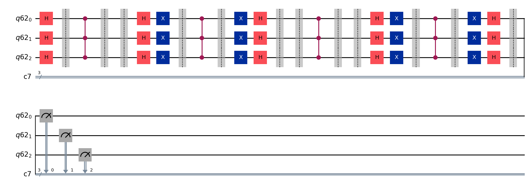
# Measure the circuit
grover_circuit.measure(range(n), range(n))

# Draw the circuit
grover_circuit.draw(output="mpl")

Optimal Number of Iterations: 2

\[-0.0883883476 |000\rangle-0.0883883476 |001\rangle-0.0883883476 |010\rangle-0.0883883476 |011\rangle-0.0883883476 |100\rangle-0.0883883476 |101\rangle-0.0883883476 |110\rangle+0.9722718241 |111\rangle\]

# Simulate the circuit, no need to transpile since just base gates are used
simulator = AerSimulator()
results = simulator.run(grover_circuit).result().get_counts()
plot_histogram(results)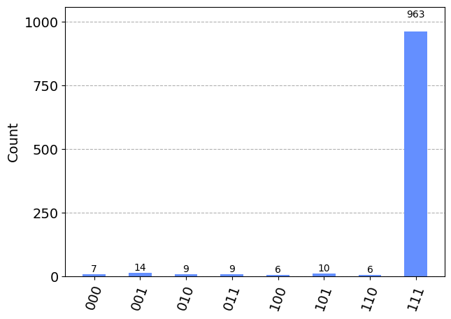

Custom Gates

To make the circuit smaller, especially since we could possible iterate through the algorithm many times, Qiskit allows us to create custom gates.

def grover_oracle_gate(num_qubits, marked_states):
    """
        Create a Grover's algorithm oracle for the general case of finding some number
        of marked strings from a list of all possible binary strings fo a given length.
        Inputs:
            num_qubits (an int): The number of qubits in the circuit
            marked_states (a list): the states to mark for the grover's Algorithm to find
        Returns:
            qc (a qiskit quantum circuit): the Grover's oracle as a single gate
    """
    # Create a quantum circuit to hold the oracle gates
    # Use the name keyword to set the name of the compound gate that will
    # eventually be returned
    qc = QuantumCircuit(num_qubits, name="Oracle")
    
    
    # Mark each target state in the input list
    for target in marked_states:
        
        # Flip target bit-string to match Qiskit bit-ordering
        rev_target = target[::-1]
        
        # Find the indices of all the '0' elements in bit-string
        # NOT gate will be placed at these values
        # NOTE ERRORS OUT IF NO 0 STATES FOUND IN STATE FIX THIS
        zero_inds = [ind for ind in range(num_qubits) if rev_target.startswith("0", ind)]
        
        # Add a multi-controlled Z-gate with pre- and post-applied X-gates (open-controls)
        # where the target bit-string has a '0' entry
        # Try/Except statement handles the case when one of the marked strings does not contain
        # any zeros
        try:
            qc.x(zero_inds)
        except:
            None
            
        # Create a multi-controlled Z-gate where the very last qubit is the target qubit
        # and all other qubits are the control qubits
        qc.compose(MCMT(ZGate(), num_qubits - 1, 1), inplace=True)
        
        
        try:
            qc.x(zero_inds)
        except:
            None

    # Once all of the individual gates are added to the circuit, make the entire
    # circuit into a single gate
    qc = qc.to_gate()

    # Return the compound gate
    return qc
    

def grover_amplification_gate(num_qubits):
    qc = QuantumCircuit(n, name="Amplify")
    qc.h(range(num_qubits))
    qc.x(range(num_qubits))
    qc.compose(MCMT(ZGate(), num_qubits - 1, 1), inplace=True)
    qc.x(range(num_qubits))
    qc.h(range(num_qubits))
    qc.barrier()
    return qc

marked_states = ["01"]

n = len(marked_states[0])
print(n)
q = QuantumRegister(n)
c = ClassicalRegister(n)
grover_circuit = QuantumCircuit(q,c)

grover_circuit.h(range(n))

optimal_num_iterations = math.floor(
math.pi / (4 * math.asin(math.sqrt(len(marked_states) / 2**n)))
)
print(optimal_num_iterations)
oracle_gate = grover_oracle_gate(n, marked_states)
amplification_gate = grover_amplification_gate(n)

for i in range(optimal_num_iterations):
    grover_circuit.append(oracle_gate, range(n))
    grover_circuit.append(amplification_gate, range(n))


grover_circuit.measure(range(n), range(n))
grover_circuit.draw(output="mpl")

2
1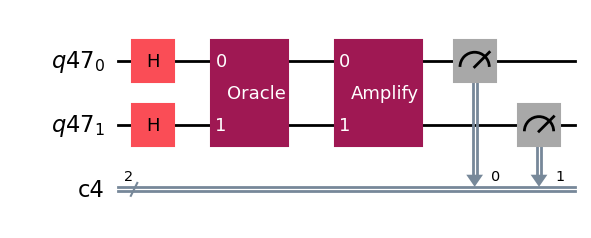

simulator = AerSimulator()
grover_circuit = transpile(grover_circuit, simulator)
results = simulator.run(grover_circuit).result().get_counts()
plot_histogram(results)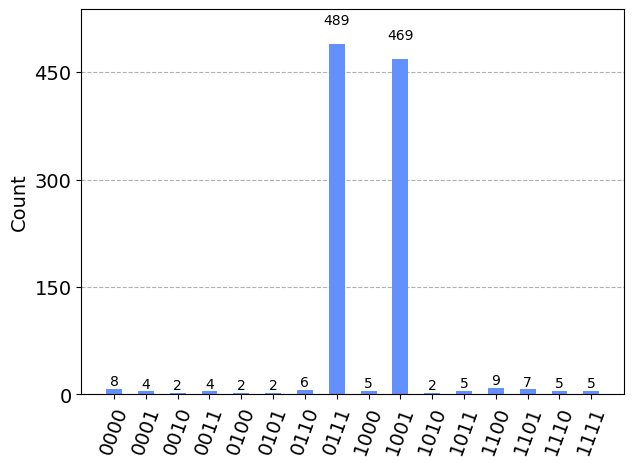

sorted_results = sorted(results, key=results.get, reverse=True)
print(marked_states)
print(sorted_results[:len(marked_states)])

['0111', '1001']
['0111', '1001']

Qiskit Built-In Functions (Amplification Only)

def grover_oracle_qiskit(marked_states):
    """Build a Grover oracle for multiple marked states

    Here we assume all input marked states have the same number of bits

    Parameters:
        marked_states (str or list): Marked states of oracle

    Returns:
        QuantumCircuit: Quantum circuit representing Grover oracle
    """
    if not isinstance(marked_states, list):
        marked_states = [marked_states]
    # Compute the number of qubits in circuit
    num_qubits = len(marked_states[0])

    qc = QuantumCircuit(num_qubits)
    # Mark each target state in the input list
    for target in marked_states:
        # Flip target bit-string to match Qiskit bit-ordering
        rev_target = target[::-1]
        # Find the indices of all the '0' elements in bit-string
        zero_inds = [ind for ind in range(num_qubits) if rev_target.startswith("0", ind)]
        # Add a multi-controlled Z-gate with pre- and post-applied X-gates (open-controls)
        # where the target bit-string has a '0' entry
        qc.x(zero_inds)
        qc.compose(MCMT(ZGate(), num_qubits - 1, 1), inplace=True)
        qc.x(zero_inds)
    return qc

marked_states = ["01111", "10000"]

oracle = grover_oracle_qiskit(marked_states)
grover_op = GroverOperator(oracle)
grover_op.decompose().draw(output="mpl")

# Note that in our implementations we took advantage of the 
# fact that Z = HXH to replace the single Hadamard, multi-control NOT gate
# single Hadamard circuit with just a multicontrol Z circuit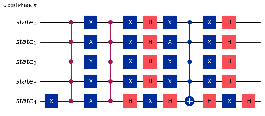

optimal_num_iterations = math.floor(
    math.pi / (4 * math.asin(math.sqrt(len(marked_states) / 2**grover_op.num_qubits)))
)

qc = QuantumCircuit(grover_op.num_qubits)
# Create even superposition of all basis states
qc.h(range(grover_op.num_qubits))
# Apply Grover operator the optimal number of times
qc.compose(grover_op.power(optimal_num_iterations), inplace=True)
# Measure all qubits
qc.measure_all()
qc.draw(output="mpl", style="iqp")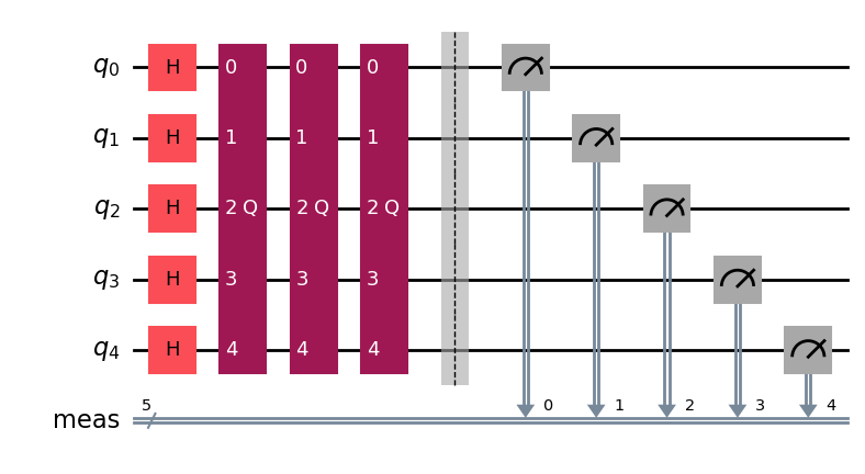

simulator = AerSimulator()
qc = transpile(qc, simulator)
results = simulator.run(qc).result().get_counts()
plot_histogram(results)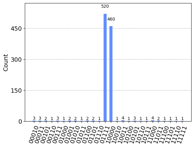

Slide Figures

states = ["00", "01", "10", "11"]
amps = (1/np.sqrt(len(states)))*np.ones(len(states))

average_amp = np.average(amps)

choice_state = "11"
choice_index = len(states)-1

plt.bar(states, amps, color="darkblue")
plt.bar(choice_index, amps[choice_index], color="darkred", label="Choice State")
plt.hlines(average_amp, 0-0.5, len(states)-1+0.5, color="darkgreen", linestyle="--", linewidth=3, label="Average Amplitude")
plt.xticks(fontfamily="serif")
plt.yticks(fontfamily="serif")
plt.xlabel("States", fontsize=14, fontfamily="serif")
plt.ylabel("Amplitude", fontsize=14, fontfamily="serif")
plt.legend(prop={'family':"serif", 'size':12}, loc=(1.01, 0.4))
# Save the image
plt.savefig("grover_vis_1.png", dpi=1000, bbox_inches="tight")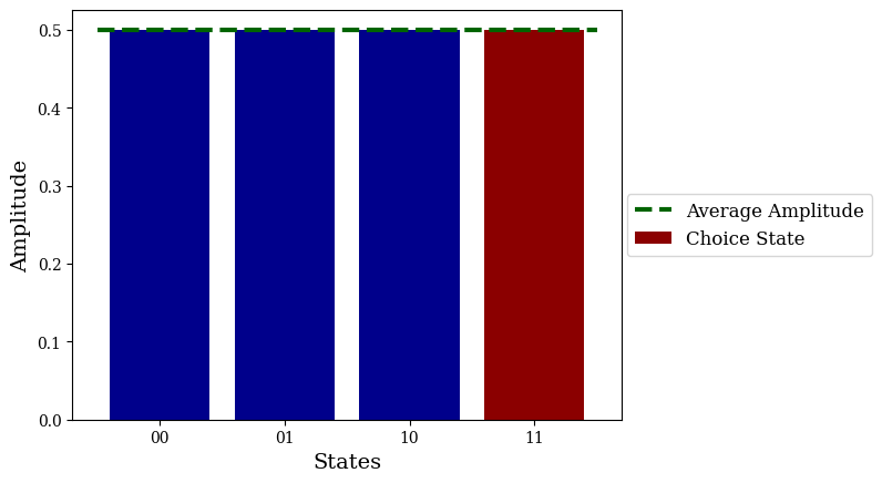

amps[choice_index] *= -1
average_amp = np.average(amps)


plt.bar(states, amps, color="darkblue")
plt.bar(choice_index, amps[choice_index], color="darkred", label="Choice State")
plt.hlines(average_amp, 0-0.5, len(states)-1+0.5, color="darkgreen", linestyle="--", linewidth=3, label="Average Amplitude")
plt.hlines(0, -1, len(states), color="black")
plt.xlim(-1, len(states))
plt.xticks(fontfamily="serif")
plt.yticks(fontfamily="serif")
plt.xlabel("States", fontsize=14, fontfamily="serif")
plt.ylabel("Amplitude", fontsize=14, fontfamily="serif")
plt.legend(prop={'family':"serif", 'size':12}, loc=(1.01, 0.4))

# Save the image
plt.savefig("grover_vis_2.png", dpi=1000, bbox_inches="tight")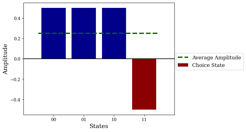

amps -= average_amp
amps = np.abs(amps)

plt.bar(states, amps, color="darkblue")
plt.bar(choice_index, amps[choice_index], color="darkred", label="Choice State")
plt.hlines(average_amp, 0-0.5, len(states)-1+0.5, color="darkgreen", linestyle="--", linewidth=3, label="Average Amplitude")
plt.hlines(0, -1, len(states), color="black")
plt.xlim(-1, len(states))
plt.xticks(fontfamily="serif")
plt.yticks(fontfamily="serif")
plt.xlabel("States", fontsize=14, fontfamily="serif")
plt.ylabel("Amplitude", fontsize=14, fontfamily="serif")
plt.legend(prop={'family':"serif", 'size':12}, loc=(1.01, 0.4))

# Save the image
plt.savefig("grover_vis_3.png", dpi=1000, bbox_inches="tight")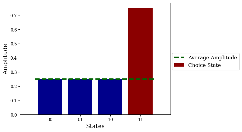

amps[choice_index] *= -1
average_amp = np.average(amps)

plt.bar(states, amps, color="darkblue")
plt.bar(choice_index, amps[choice_index], color="darkred", label="Choice State")
plt.hlines(average_amp, 0-0.5, len(states)-1+0.5, color="darkgreen", linestyle="--", linewidth=3, label="Average Amplitude")
plt.hlines(0, -1, len(states), color="black")
plt.xlim(-1, len(states))
plt.xticks(fontfamily="serif")
plt.yticks(fontfamily="serif")
plt.xlabel("States", fontsize=14, fontfamily="serif")
plt.ylabel("Amplitude", fontsize=14, fontfamily="serif")
plt.legend(prop={'family':"serif", 'size':12}, loc=(1.01, 0.4))

# Save the image
plt.savefig("grover_vis_4.png", dpi=1000, bbox_inches="tight")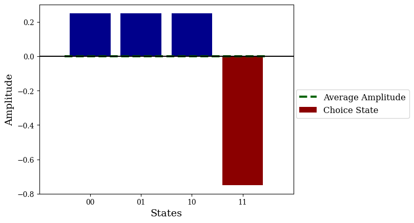

amps -= average_amp
amps = np.abs(amps)

plt.bar(states, amps, color="darkblue")
plt.bar(choice_index, amps[choice_index], color="darkred", label="Choice State")
plt.hlines(average_amp, 0-0.5, len(states)-1+0.5, color="darkgreen", linestyle="--", linewidth=3, label="Average Amplitude")
plt.hlines(0, -1, len(states), color="black")
plt.xlim(-1, len(states))
plt.xticks(fontfamily="serif")
plt.yticks(fontfamily="serif")
plt.xlabel("States", fontsize=14, fontfamily="serif")
plt.ylabel("Amplitude", fontsize=14, fontfamily="serif")
plt.legend(prop={'family':"serif", 'size':12}, loc=(1.01, 0.4))

# Save the image
plt.savefig("grover_vis_5.png", dpi=1000, bbox_inches="tight")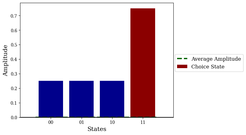

qc = QuantumCircuit(1)

qc.x(0)
qc.h(0)

qc.draw(output="mpl")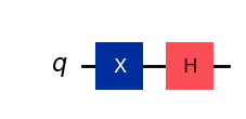

# Create a single vector
V = np.array([3,4])

# Create the plot
fig, ax = plt.subplots()

# Add the vector V to the plot
ax.quiver(0, 0, V[0], V[1], angles='xy', scale_units='xy', scale=1, color='r')

plt.xlim(-5,5)
plt.ylim(-5,5)

# using 'spines', new in Matplotlib 1.0
ax.spines['left'].set_position('zero')
ax.spines['right'].set_color('none')
ax.spines['bottom'].set_position('zero')
ax.spines['top'].set_color('none')
ax.xaxis.set_ticks_position('bottom')
ax.yaxis.set_ticks_position('left')

# Show the plot along with the grid
plt.grid(which="both")
plt.savefig("reflection1.png", dpi=1000)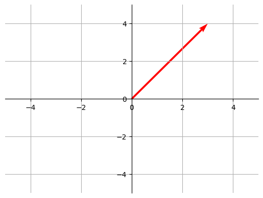

# Create a single vector
V = np.array([3,4])
V2 = np.array([3,-4])

# Create the plot
fig, ax = plt.subplots()

# Add the vector V to the plot
ax.quiver(0, 0, V[0], V[1], angles='xy', scale_units='xy', scale=1, color='r')
ax.quiver(0, 0, V2[0], V2[1], angles='xy', scale_units='xy', scale=1, color='r')

plt.xlim(-5,5)
plt.ylim(-5,5)

# using 'spines', new in Matplotlib 1.0
ax.spines['left'].set_position('zero')
ax.spines['right'].set_color('none')
ax.spines['bottom'].set_position('zero')
ax.spines['top'].set_color('none')
ax.xaxis.set_ticks_position('bottom')
ax.yaxis.set_ticks_position('left')

# Show the plot along with the grid
plt.grid(which="both")
plt.savefig("reflection2.png", dpi=1000)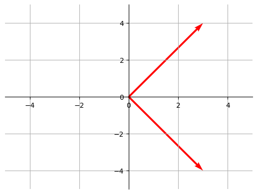

# Create a single vector
V = np.array([3,4])
V2 = np.array([3,-4])
V3 = np.array([0,-4])

# Create the plot
fig, ax = plt.subplots()

# Add the vector V to the plot
ax.quiver(0, 0, V[0], V[1], angles='xy', scale_units='xy', scale=1, color='r')
ax.quiver(0, 0, V2[0], V2[1], angles='xy', scale_units='xy', scale=1, color='r')
ax.quiver(3, 4, V3[0], V3[1], angles='xy', scale_units='xy', scale=1, color='b')
ax.quiver(3, 0, V3[0], V3[1], angles='xy', scale_units='xy', scale=1, color='b')


plt.xlim(-5,5)
plt.ylim(-5,5)

# using 'spines', new in Matplotlib 1.0
ax.spines['left'].set_position('zero')
ax.spines['right'].set_color('none')
ax.spines['bottom'].set_position('zero')
ax.spines['top'].set_color('none')
ax.xaxis.set_ticks_position('bottom')
ax.yaxis.set_ticks_position('left')

# Show the plot along with the grid
plt.grid(which="both")
plt.savefig("reflection3.png", dpi=1000)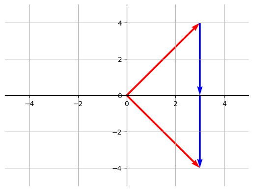

down = np.array([0,1])
down_down = np.kron(down, down)
outer = np.outer(down_down, down_down)
U = np.eye(4) - outer

outer

array([[0, 0, 0, 0],
       [0, 0, 0, 0],
       [0, 0, 0, 0],
       [0, 0, 0, 1]])

fig, ax = plt.subplots()
# Create a single vector
s = np.array([0,1])
phi = np.array([12/13,5/13])
s_per = np.array([0,-4])

plt.hlines(0, -1.1, 1.1, color="black", linewidth=0.5)
plt.vlines(0, -1.1, 1.1, color="black", linewidth=0.5)

# Add the vector V to the plot
ax.quiver(0, 0, s[0], s[1], angles='xy', scale_units='xy', scale=1, color='r', label="s", linewidth=2)
ax.quiver(0, 0, phi[0], phi[1], angles='xy', scale_units='xy', scale=1, color='b', label=r"\phi", linewidth=2)



circ = plt.Circle((0, 0), radius=1, edgecolor='black', facecolor='None')
plt.xlim(-1.1,1.1)
plt.ylim(-1.1,1.1)
plt.grid(which="both")
ax.add_patch(circ)
plt.legend()
ax.set_aspect('equal', adjustable='box')
plt.savefig("grovercircle1.png", dpi=1000)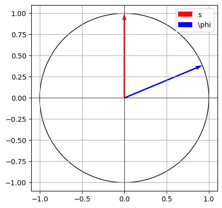

fig, ax = plt.subplots()
# Create a single vector
s = np.array([0,1])
phi = np.array([12/13,5/13])
s_per = np.array([1,0])


circ = plt.Circle((0, 0), radius=1, edgecolor='black', facecolor='None')
ax.add_patch(circ)


plt.hlines(0, -1.1, 1.1, color="black", linewidth=0.5)
plt.vlines(0, -1.1, 1.1, color="black", linewidth=0.5)

# Add the vector V to the plot
ax.quiver(0, 0, s[0], s[1], angles='xy', scale_units='xy', scale=1, color='r', label="s", linewidth=2)
ax.quiver(0, 0, phi[0], phi[1], angles='xy', scale_units='xy', scale=1, color='b', label=r"\phi", linewidth=2)
ax.quiver(0, 0, s_per[0], s_per[1], angles='xy', scale_units='xy', scale=1, color='g', label=r"s_perpen.", linewidth=2)


plt.xlim(-1.1,1.1)
plt.ylim(-1.1,1.1)
plt.grid(which="both")
plt.legend(loc=(1.01, 0.4))
ax.set_aspect('equal', adjustable='box')
plt.savefig("grovercircle2.png", dpi=1000, bbox_inches="tight")

fig, ax = plt.subplots()
# Create a single vector
s = np.array([0,1])
phi = np.array([12/13,5/13])
s_per = np.array([1,0])

plt.hlines(0, -1.1, 1.1, color="black", linewidth=0.5)
plt.vlines(0, -1.1, 1.1, color="black", linewidth=0.5)

# Add the vector V to the plot
ax.quiver(0, 0, s[0], s[1], angles='xy', scale_units='xy', scale=1, color='r', label="s", linewidth=2)
ax.quiver(0, 0, phi[0], phi[1], angles='xy', scale_units='xy', scale=1, color='b', label=r"\phi", linewidth=2)
ax.quiver(0, 0, s_per[0], s_per[1], angles='xy', scale_units='xy', scale=1, color='g', label=r"s_perpen.", linewidth=2)

y = 5/13
x = 12/13

angle_rad = np.arctan2(y, x)
angle_deg = np.degrees(angle_rad)

arc = np.linspace(0, angle_rad, 100)
arc_x = np.cos(arc)/4
arc_y = np.sin(arc)/4
ax.plot(arc_x, arc_y, 'black')
ax.text(0.4, 0.05, f'θ', fontsize=14, color='black')

circ = plt.Circle((0, 0), radius=1, edgecolor='black', facecolor='None')
plt.xlim(-1.1,1.1)
plt.ylim(-1.1,1.1)
plt.grid(which="both")
ax.add_patch(circ)
plt.legend(loc=(1.01, 0.4))
ax.set_aspect('equal', adjustable='box')
plt.savefig("grovercircle3.png", dpi=1000, bbox_inches="tight")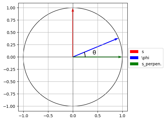

fig, ax = plt.subplots()
# Create a single vector
s = np.array([0,1])
phi = np.array([12/13,5/13])
s_per = np.array([1,0])

plt.hlines(0, -1.1, 1.1, color="black", linewidth=0.5)
plt.vlines(0, -1.1, 1.1, color="black", linewidth=0.5)

# Add the vector V to the plot
ax.quiver(0, 0, s[0], s[1], angles='xy', scale_units='xy', scale=1, color='r', label="s", linewidth=2)
ax.quiver(0, 0, phi[0], phi[1], angles='xy', scale_units='xy', scale=1, color='b', label=r"\phi", linewidth=2)
ax.quiver(0, 0, s_per[0], s_per[1], angles='xy', scale_units='xy', scale=1, color='g', label=r"s_perpen.", linewidth=2)
ax.quiver(0, 0, phi[0], -phi[1], angles='xy', scale_units='xy', scale=1, color='purple', linewidth=2, label="Oracle 1")

y = 5/13
x = 12/13

angle_rad = np.arctan2(y, x)
angle_deg = np.degrees(angle_rad)

arc = np.linspace(0, angle_rad, 100)
arc_x = np.cos(arc)/4
arc_y = np.sin(arc)/4
ax.plot(arc_x, arc_y, 'black')
ax.text(0.4, 0.05, f'θ', fontsize=14, color='black')

arc = np.linspace(0, angle_rad, 100)
arc_x = np.cos(arc)/4
arc_y = -np.sin(arc)/4
ax.plot(arc_x, arc_y, 'black')
ax.text(0.4, -0.14, f'θ', fontsize=14, color='black')

circ = plt.Circle((0, 0), radius=1, edgecolor='black', facecolor='None')
plt.xlim(-1.1,1.1)
plt.ylim(-1.1,1.1)
plt.grid(which="both")
ax.add_patch(circ)
plt.legend(loc=(1.01, 0.4))
ax.set_aspect('equal', adjustable='box')
plt.savefig("grovercircle4.png", dpi=1000, bbox_inches="tight")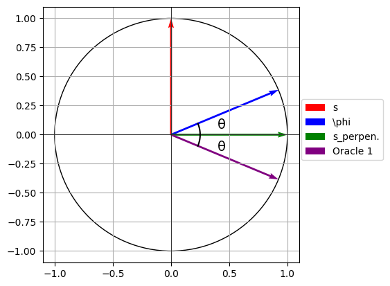

fig, ax = plt.subplots()
# Create a single vector
s = np.array([0,1])
phi = np.array([12/13,5/13])
s_per = np.array([1,0])

plt.hlines(0, -1.1, 1.1, color="black", linewidth=0.5)
plt.vlines(0, -1.1, 1.1, color="black", linewidth=0.5)

# Add the vector V to the plot
ax.quiver(0, 0, s[0], s[1], angles='xy', scale_units='xy', scale=1, color='r', label="s", linewidth=2)
ax.quiver(0, 0, phi[0], phi[1], angles='xy', scale_units='xy', scale=1, color='b', label=r"\phi", linewidth=2)
ax.quiver(0, 0, s_per[0], s_per[1], angles='xy', scale_units='xy', scale=1, color='g', label=r"s_perpen.", linewidth=2)
ax.quiver(0, 0, phi[0], -phi[1], angles='xy', scale_units='xy', scale=1, color='purple', linewidth=2, label="Oracle 1")



y = 5/13
x = 12/13

angle_rad = np.arctan2(y, x)
angle_deg = np.degrees(angle_rad)

dif1 = np.array([np.cos(3*angle_rad), np.sin(3*angle_rad)]) 

ax.quiver(0, 0, dif1[0], dif1[1], angles='xy', scale_units='xy', scale=1, color='slategrey', linewidth=2, label="Amplify 1")


arc = np.linspace(0, angle_rad, 100)
arc_x = np.cos(arc)/4
arc_y = np.sin(arc)/4
ax.plot(arc_x, arc_y, 'black')
ax.text(0.4, 0.05, f'θ', fontsize=14, color='black')

arc = np.linspace(0, angle_rad, 100)
arc_x = np.cos(arc)/4
arc_y = -np.sin(arc)/4
ax.plot(arc_x, arc_y, 'black')
ax.text(0.4, -0.14, f'θ', fontsize=14, color='black')

arc = np.linspace(0, 3*angle_rad, 100)
arc_x = np.cos(arc)/2
arc_y = np.sin(arc)/2
ax.plot(arc_x, arc_y, 'black')
ax.text(0.45, 0.4, f'3θ', fontsize=14, color='black')

circ = plt.Circle((0, 0), radius=1, edgecolor='black', facecolor='None')
plt.xlim(-1.1,1.1)
plt.ylim(-1.1,1.1)
plt.grid(which="both")
ax.add_patch(circ)
plt.legend(loc=(1.01, 0.4))
ax.set_aspect('equal', adjustable='box')
plt.savefig("grovercircle5.png", dpi=1000, bbox_inches="tight")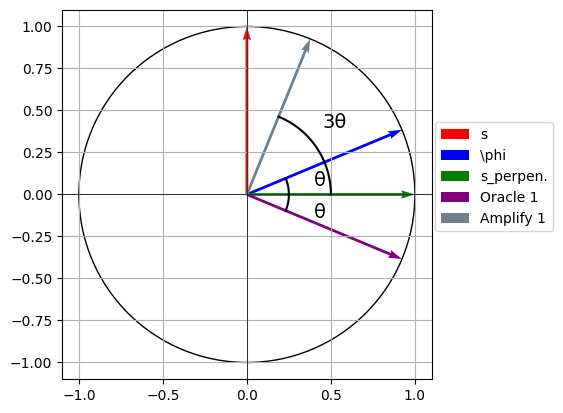

fig, ax = plt.subplots()
# Create a single vector
s = np.array([0,1])
phi = np.array([12/13,5/13])
s_per = np.array([1,0])

plt.hlines(0, -1.1, 1.1, color="black", linewidth=0.5)
plt.vlines(0, -1.1, 1.1, color="black", linewidth=0.5)

# Add the vector V to the plot
ax.quiver(0, 0, s[0], s[1], angles='xy', scale_units='xy', scale=1, color='r', label="s", linewidth=2)
ax.quiver(0, 0, phi[0], phi[1], angles='xy', scale_units='xy', scale=1, color='b', label=r"\phi", linewidth=2)
ax.quiver(0, 0, s_per[0], s_per[1], angles='xy', scale_units='xy', scale=1, color='g', label=r"s_perpen.", linewidth=2)
ax.quiver(0, 0, phi[0], -phi[1], angles='xy', scale_units='xy', scale=1, color='purple', linewidth=2, label="Oracle 1")



y = 5/13
x = 12/13

angle_rad = np.arctan2(y, x)
angle_deg = np.degrees(angle_rad)

dif1 = np.array([np.cos(3*angle_rad), np.sin(3*angle_rad)]) 

ax.quiver(0, 0, dif1[0], dif1[1], angles='xy', scale_units='xy', scale=1, color='slategrey', linewidth=2, label="Amplify 1")
ax.quiver(0, 0, dif1[0], -dif1[1], angles='xy', scale_units='xy', scale=1, color='darkorange', linewidth=2, label="Oracle 2")


arc = np.linspace(0, angle_rad, 100)
arc_x = np.cos(arc)/4
arc_y = np.sin(arc)/4
ax.plot(arc_x, arc_y, 'black')
ax.text(0.4, 0.05, f'θ', fontsize=14, color='black')

arc = np.linspace(0, angle_rad, 100)
arc_x = np.cos(arc)/4
arc_y = -np.sin(arc)/4
ax.plot(arc_x, arc_y, 'black')
ax.text(0.4, -0.14, f'θ', fontsize=14, color='black')

arc = np.linspace(0, 3*angle_rad, 100)
arc_x = np.cos(arc)/2
arc_y = np.sin(arc)/2
ax.plot(arc_x, arc_y, 'black')
ax.text(0.45, 0.4, f'3θ', fontsize=14, color='black')

arc = np.linspace(0, 3*angle_rad, 100)
arc_x = np.cos(arc)/2
arc_y = -np.sin(arc)/2
ax.plot(arc_x, arc_y, 'black')
ax.text(0.45, -0.45, f'3θ', fontsize=14, color='black')

circ = plt.Circle((0, 0), radius=1, edgecolor='black', facecolor='None')
plt.xlim(-1.1,1.1)
plt.ylim(-1.1,1.1)
plt.grid(which="both")
ax.add_patch(circ)
plt.legend(loc=(1.01, 0.4))
ax.set_aspect('equal', adjustable='box')
plt.savefig("grovercircle6.png", dpi=1000, bbox_inches="tight")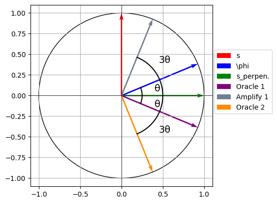

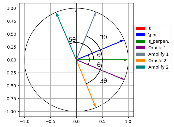
fig, ax = plt.subplots()
# Create a single vector
s = np.array([0,1])
phi = np.array([12/13,5/13])
s_per = np.array([1,0])

plt.hlines(0, -1.1, 1.1, color="black", linewidth=0.5)
plt.vlines(0, -1.1, 1.1, color="black", linewidth=0.5)

# Add the vector V to the plot
ax.quiver(0, 0, s[0], s[1], angles='xy', scale_units='xy', scale=1, color='r', label="s", linewidth=2)
ax.quiver(0, 0, phi[0], phi[1], angles='xy', scale_units='xy', scale=1, color='b', label=r"\phi", linewidth=2)
ax.quiver(0, 0, s_per[0], s_per[1], angles='xy', scale_units='xy', scale=1, color='g', label=r"s_perpen.", linewidth=2)
ax.quiver(0, 0, phi[0], -phi[1], angles='xy', scale_units='xy', scale=1, color='purple', linewidth=2, label="Oracle 1")



y = 5/13
x = 12/13

angle_rad = np.arctan2(y, x)
angle_deg = np.degrees(angle_rad)

dif1 = np.array([np.cos(3*angle_rad), np.sin(3*angle_rad)]) 

ax.quiver(0, 0, dif1[0], dif1[1], angles='xy', scale_units='xy', scale=1, color='slategrey', linewidth=2, label="Amplify 1")
ax.quiver(0, 0, dif1[0], -dif1[1], angles='xy', scale_units='xy', scale=1, color='darkorange', linewidth=2, label="Oracle 2")


dif2 = np.array([np.cos(5*angle_rad), np.sin(5*angle_rad)]) 
ax.quiver(0, 0, dif2[0], dif2[1], angles='xy', scale_units='xy', scale=1, color='teal', linewidth=2, label="Amplify 2")


arc = np.linspace(0, angle_rad, 100)
arc_x = np.cos(arc)/4
arc_y = np.sin(arc)/4
ax.plot(arc_x, arc_y, 'black')
ax.text(0.4, 0.05, f'θ', fontsize=14, color='black')

arc = np.linspace(0, angle_rad, 100)
arc_x = np.cos(arc)/4
arc_y = -np.sin(arc)/4
ax.plot(arc_x, arc_y, 'black')
ax.text(0.4, -0.14, f'θ', fontsize=14, color='black')

arc = np.linspace(0, 3*angle_rad, 100)
arc_x = np.cos(arc)/2
arc_y = np.sin(arc)/2
ax.plot(arc_x, arc_y, 'black')
ax.text(0.45, 0.4, f'3θ', fontsize=14, color='black')

arc = np.linspace(0, 3*angle_rad, 100)
arc_x = np.cos(arc)/2
arc_y = -np.sin(arc)/2
ax.plot(arc_x, arc_y, 'black')
ax.text(0.45, -0.45, f'3θ', fontsize=14, color='black')

arc = np.linspace(0, 5*angle_rad, 100)
arc_x = np.cos(arc)/3
arc_y = np.sin(arc)/3
ax.plot(arc_x, arc_y, 'black')
ax.text(-0.15, 0.35, f'5θ', fontsize=14, color='black')

circ = plt.Circle((0, 0), radius=1, edgecolor='black', facecolor='None')
plt.xlim(-1.1,1.1)
plt.ylim(-1.1,1.1)
plt.grid(which="both")
ax.add_patch(circ)
plt.legend(loc=(1.01, 0.4))
ax.set_aspect('equal', adjustable='box')
plt.savefig("grovercircle7.png", dpi=1000, bbox_inches="tight")