from qiskit import QuantumRegister, QuantumCircuit, ClassicalRegister
from qiskit_aer import AerSimulator

import numpy as npVariational Quantum Eigensolver (VQE)
def pairing_2p2h (g,d):
    return np.array([[-g/2, 0], [0, 2*d-g/2]])


H = pairing_2p2h(0.5, 1)

print("Hamiltonian")
print(H)
print("Adjoint of Hamiltonian")
print(H.conj().T)
print()

print("Is the Hamiltonian Hermitian?")
print(H == H.conj().T)
print()

print("Hamiltonian Multiplied by Adjoint")
print(H.dot(H.conj().T))
print()

print("Is the Hamiltonian Unitary?")
print(H.dot(H.conj().T) == np.eye(2))
Hamiltonian
[[-0.25 0. ]
[ 0. 1.75]]
Adjoint of Hamiltonian
[[-0.25 0. ]
[ 0. 1.75]]
Is the Hamiltonian Hermitian?
[[ True True]
[ True True]]
Hamiltonian Multiplied by Adjoint
[[0.0625 0. ]
[0. 3.0625]]
Is the Hamiltonian Unitary?
[[False True]
[ True False]]def pairing_4p4h(g,d):
return np.array([
[2*d-g, -g/2, -g/2, -g/2, -g/2, 0],
[-g/2, 4*d-g, -g/2, -g/2, 0, -g/2],
[-g/2, -g/2, 6*d-g, 0, -g/2, -g/2],
[-g/2, -g/2, 0, 6*d-g, -g/2, -g/2],
[-g/2, 0, -g/2, -g/2, 8*d-g, -g/2],
[0, -g/2, -g/2, -g/2, -g/2, 10*d-g]
])
g = 0.5
d = 1.0
energies, states = np.linalg.eig(pairing_4p4h(g,d))
states = states.T
for i in range(len(energies)):
print("Energy:", energies[i])
print("State:", states[i])
print("Normalized?", np.linalg.norm(states[i]))
print()Energy: 1.416774284351102
State: [-0.98419512 -0.13663267 -0.07210914 -0.07210914 -0.04679042 -0.01013337]
Normalized? 1.0
Energy: 3.4706732152562574
State: [-0.1521038 0.97511354 0.10838838 0.10838838 0.0070972 0.04971482]
Normalized? 0.9999999999999999
Energy: 5.499999999999999
State: [-0.08512565 -0.17025131 0.68100522 0.68100522 0.17025131 0.08512565]
Normalized? 0.9999999999999999
Energy: 7.549436759324765
State: [ 0.03029686 -0.01194329 0.12855978 0.12855978 -0.97829206 -0.09396206]
Normalized? 1.0
Energy: 9.563115741067884
State: [-0.00775438 0.03683671 0.05250236 0.05250236 0.10825629 -0.99063137]
Normalized? 0.9999999999999999
Energy: 5.500000000000002
State: [ 0.01490915 0.02981829 0.57690389 -0.81545023 -0.02981829 -0.01490915]
Normalized? 1.0
q = QuantumRegister(4)
c = ClassicalRegister(4)
qc = QuantumCircuit(q,c)

qc.x([0,1])

qc.draw(output="mpl")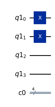
q = QuantumRegister(4)
c = ClassicalRegister(4)
qc = QuantumCircuit(q,c)

qc.x([0,2])

qc.draw(output="mpl")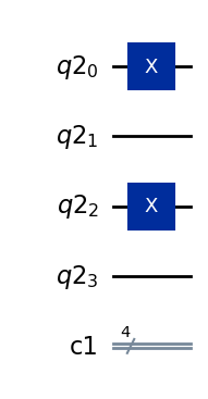
q = QuantumRegister(4)
c = ClassicalRegister(4)
qc = QuantumCircuit(q,c)

qc.x([2,3])

qc.draw(output="mpl")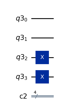
VQE With a Test System
## Definitions

# Pi
pi = np.pi

# The up and down qubits
up = np.matrix([[1],[0]],dtype=complex)
down  = np.matrix([[0],[1]],dtype=complex)

# Defining some relevant quantum gate matrices
# Spefically the Pauli matrices
I = np.matrix([[1,0],[0,1]],dtype=complex)
X = np.matrix([[0,1],[1,0]],dtype=complex)
Y = np.matrix([[0,-1j],[1j,0]],dtype=complex)
Z = np.matrix([[1,0],[0,-1]],dtype=complex)
# 1. **Hamiltonian Preparation:** Define the Hamiltonian of the system then write it in terms of the Pauli operators.
# Define the Hamiltonian of the test system in terms of the Pauli matrices
def hamiltonian(A):
return (A/2)*(np.kron(X,X) + np.kron(Y,Y))
# Print a test version of the Hamiltonian
A = 1
H = hamiltonian(A)
print(H)[[0.+0.j 0.+0.j 0.+0.j 0.+0.j]
[0.+0.j 0.+0.j 1.+0.j 0.+0.j]
[0.+0.j 1.+0.j 0.+0.j 0.+0.j]
[0.+0.j 0.+0.j 0.+0.j 0.+0.j]]# Define and print the four two-qubit states
state_00 = np.kron(up, up)
state_01 = np.kron(up, down)
state_10 = np.kron(down, up)
state_11 = np.kron(down, down)
print("00:\n", state_00, "\n")
print("01:\n", state_01, "\n")
print("10:\n", state_10, "\n")
print("11:\n", state_11, "\n")00:
[[1.+0.j]
[0.+0.j]
[0.+0.j]
[0.+0.j]]
01:
[[0.+0.j]
[1.+0.j]
[0.+0.j]
[0.+0.j]]
10:
[[0.+0.j]
[0.+0.j]
[1.+0.j]
[0.+0.j]]
11:
[[0.+0.j]
[0.+0.j]
[0.+0.j]
[1.+0.j]]
# Apply the Hamiltonian to the four states
# Note that only two of them give a non-zero results
# So a good attempt to create the trial wavefunction likely will
# involve the |01> and |10> states.
print("H|00>:\n", H@state_00, "\n")
print("H|01>:\n", H@state_01, "\n")
print("H|10>:\n", H@state_10, "\n")
print("H|11>:\n", H@state_11, "\n")
H|00>:
[[0.+0.j]
[0.+0.j]
[0.+0.j]
[0.+0.j]]
H|01>:
[[0.+0.j]
[0.+0.j]
[1.+0.j]
[0.+0.j]]
H|10>:
[[0.+0.j]
[1.+0.j]
[0.+0.j]
[0.+0.j]]
H|11>:
[[0.+0.j]
[0.+0.j]
[0.+0.j]
[0.+0.j]]
# These gates need to be applied to the quantum circuit to measure the YY portion
# of the Hamiltonian
# Note that Y = SXS_dag = SHZHS_dag, so we are taking the final two matrices of this
# expansion and applying them in reverse order (the two matrices after the Z gate).
def r_yy ():
    q = QuantumRegister(2)
    c = ClassicalRegister(2)
    qc = QuantumCircuit(q,c)

    qc.sdg(range(2))
    qc.h(range(2))

    return qc

# These gates are needed to measure the XX portion of the Hamiltonian.
# X = HZH, we we are taking the final gate, the one after the Z
def r_xx ():
    q = QuantumRegister(2)
    c = ClassicalRegister(2)
    qc = QuantumCircuit(q,c)

    qc.h(range(2))

    return qc
# 2. **Create an Ansatz**: Create an iniital guess for the ground state of the quantum system,
# called an ansatz. It must be parameterized by a series of parameters called $\theta$.
# It can be hardware inspired or physically inspired.
# The below function creates the trial wavefunction proposed in the slides.
def ansatz(theta):
# create two-qubit quantum register
q = QuantumRegister(2,'q')
c = ClassicalRegister(2,'c')
# initialize quantum circuit
qc = QuantumCircuit(q,c)
# Apply phase shifts based on the desired phases for each state
qc.h(0)
qc.x(1)
qc.cx(0,1)
qc.p(theta,1)
# return circuit
return qc
# Let's check to see that we are creating the correct function
from qiskit.quantum_info import Statevector

wavefunction = ansatz(pi/3)

statevector = Statevector(wavefunction)
display(statevector.draw(output = 'latex'))
\[\frac{\sqrt{2}}{2} |01\rangle+(\frac{\sqrt{2}}{4} + \frac{\sqrt{6} i}{4}) |10\rangle\]
# The below function computes the expectation value given the simultions of a
# quantum circuit using the Hamming weight formula presented in the slides.

## expecation value
def counts_to_exp(counts):

    # populate empty counts with 0
    for bs in ['00','01','10','11']:
        if bs not in counts:
            counts[bs] = 0

    # numerator of expecation value
    num = counts['00'] - counts['01'] - counts['10'] + counts['11']

    # denominator of expectation value
    den = counts['00'] + counts['01'] + counts['10'] + counts['11']

    # expectation value
    exp = num/den

    return exp
# expecation value of the Hamiltonian
def exp_of_H(theta,A):
# 3. **Prepare the Quantum Circuit:** Initialize the quantum system into a simple r
# eference state and then apply the ansatz with specific values for $\theta$.
# The Hamiltonian is then "added" to the circuit using its Pauli operator form
# generated in step 1.
# prepare ansatz, one per expectation value
circ_xx = ansatz(theta)
circ_yy = ansatz(theta)
# Add the appropriate gates for each expectation value
circ_xx.compose(r_xx(), range(2), inplace=True)
circ_yy.compose(r_yy(), range(2), inplace=True)
# 4. **Measure the Expectation Value:** Run the circuit many times and get a
# measurement for each one. This is an estimation for the energy with the given
# set of parameters $\theta$.
# measure each circuit
circ_xx.measure(circ_xx.qubits,circ_xx.clbits)
circ_yy.measure(circ_yy.qubits,circ_yy.clbits)
# get the counts of each circuit
simulator = AerSimulator()
counts_xx = simulator.run(circ_xx).result().get_counts()
counts_yy = simulator.run(circ_yy).result().get_counts()
# get the expectation value from each set of counts
exp_xx = counts_to_exp(counts_xx)
exp_yy = counts_to_exp(counts_yy)
# get the expectation value of the Hamiltonian
exp = (A/2)*(exp_xx + exp_yy)
# return the expectation value of the Hamiltonian
return exp# Test the circuit with one particular value of theta
theta = pi/2
exp_pi_2 = exp_of_H(theta, 1)
print("The expected ground state energy is", exp_pi_2)
H = hamiltonian(1)
eig_vals, eig_vecs = np.linalg.eig(H)
ground_state_E = np.min(eig_vals).real
print("The true ground state energy is", np.round(ground_state_E, 3))The expected ground state energy is 0.005859375
The true ground state energy is -1.0# 5. **Classical Optimization**: Using a classical optimization algorithm, minimize the
# energy with repect to $\theta$.
# Here we will just use a brute force method to search through many possible values, but you
# also set up an optimization algorithm using scipy
expected_E = []
minimim_theta = None
minimum_E = 1000
for theta in np.linspace(0, 2*pi, 100):
E = exp_of_H(theta,1)
expected_E.append(E)
if E < minimum_E:
minimum_E = E
minimim_theta = theta
H = hamiltonian(1)
eig_vals, eig_vecs = np.linalg.eig(H)
ground_state_E = np.min(eig_vals).real
print("The true ground state energy is", np.round(ground_state_E, 3))
print("The lowest energy found with VQE is", np.round(minimum_E, 3))
print("The difference in the energies is", ground_state_E - minimum_E)
print("This occured at an angle of theta equal to", np.round(minimim_theta, 3))The true ground state energy is -1.0
The lowest energy found with VQE is -0.999
The difference in the energies is -0.0006510416666666297
This occured at an angle of theta equal to 3.11# Plot the results of the search
import matplotlib.pyplot as plt
plt.plot(np.linspace(0, 2*pi, 100), expected_E, linewidth=2, color="b", label="VQE Energy")
plt.hlines(-1, 0, 2*pi, color="r", linewidth=2, linestyle="--", label="True Ground State")
plt.xlabel(r"$\theta$")
plt.ylabel(r"$\langle E \rangle$")
plt.legend(loc="upper right")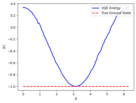
# Imports
%matplotlib inline
import matplotlib.pyplot as plt
import numpy as np
import scipy
from qiskit import QuantumCircuit, QuantumRegister, ClassicalRegister
from qiskit.circuit.library import UnitaryGate


## Definitions
pi = np.pi

I = np.matrix([[1,0],[0,1]],dtype=complex)
X = np.matrix([[0,1],[1,0]],dtype=complex)
Y = np.matrix([[0,-1j],[1j,0]],dtype=complex)
Z = np.matrix([[1,0],[0,-1]],dtype=complex)
##############################
##            SA            ##
##############################
def SA(t):
    """
        Inputs:
            t (a float): the coefficeint to be used in the exponent
        Returns:
            SA (a Qiskit Gate): a Qiskit gate consisting of the A_a^i gate and a SWAp
                gate.
        Creates one of the gates in the SWAP network for below Fermi level qubit i and
        above Fermi level qubit a. The gate is based on the equation for the ansatz with
        a SWAP after the ansatz term is applied.
    """

    # define SWAP matrix
    swap = np.array([[1,0,0,0],[0,0,1,0],[0,1,0,0],[0,0,0,1]])

    # define matrix for SA (see the lecture notes for the equation form)
    # Note that kron is the tensor product and expm is the scipy function for
    # an exponent to a matrix (need to do a Taylor expansion for the result see
    # the documentation)
    # The result of this line is a matrix.
    SA = swap @ scipy.linalg.expm(1.0j*(t/2)*(np.kron(X,Y)-np.kron(Y,X)))

    # Convert the Numpy array to a qiskit gate
    SA = UnitaryGate(SA)

    # return gate
    return SA

##############################
##          ANSATZ          ##
##############################
def ansatz(t_list):
    """
        Inputs:
            t_list (a Numpy array): a list of four numbers to be used in the exponent
                of the operator. In order, they are the coefficeints for the i = 0, a = 2
                state, the i = 0, a = 3 state, the i = 1, a = 2 state, and the i = 1, a = 3
        Returns:
            circ (a qiskit circuit): a qiskit circuit representing the ansatz of teh VQE a
                algorithm
        Prepares a quantum circuit in the ansatz for the pairing model.
    """

    # create registers
    q = QuantumRegister(4,'q')
    c = ClassicalRegister(4,'c')

    # initialize quantum circuit
    circ = QuantumCircuit(q,c)

    # prepare |Phi>, which is the Fock state or the
    # ground state in second quantization
    circ.x(q[0])
    circ.x(q[1])

    # Apply the swap network, pulling the correct coefficient from the t_list
    # for each pair of a and i values
    circ.append(SA(t_list[2]),[q[1],q[2]]) # i = 1, a = 2
    # The qubits are now in the order 0, 2, 1, 3
    # So now 0 and 2 are beside each other, 1 and 3 are beside each other
    # 0 and 2 now have indices 0 and 1 and 1 and 3 now have indices 2 and 3
    circ.append(SA(t_list[0]),[q[0],q[1]]) # i = 0, a = 2
    # The qubits are now in the order 2, 0, 1, 3
    circ.append(SA(t_list[3]),[q[2],q[3]]) # i = 1, a = 3
    # The qubits are now in the order 2, 0, 3, 1
    # So qubits 0, 3 are beside each other with indices 1 and 2
    circ.append(SA(t_list[1]),[q[1],q[2]]) # i = 0, a = 3

    # The final ordering of the qubits is 2, 0, 1, 3

    # return circuit
    return circ

##############################
##       ROTATE TO XXXX     ##
##############################
def rotate_to_xxxx(circ):
    """
        Inputs:
            circ (a qiskit circuit): a qiskit circuit set up as the ansatz
        Returns:
            circ (a qiskit circuit): the same circuit but with the gates applied
                to rotate it to measuring in the x basis.
        Applies the gates needed to measure in the x basis to all four qubits of the
        circuit.
    """
    circ.h(range(4))
    return circ

##############################
##       ROTATE TO YYYY     ##
##############################
def rotate_to_yyyy(circ):
    """
        Inputs:
            circ (a qiskit circuit): a qiskit circuit set up as the ansatz
        Returns:
            circ (a qiskit circuit): the same circuit but with the gates applied
                to rotate it to measuring in the y basis.
        Applies the gates needed to measure in the y basis to all four qubits of the
        circuit.
    """
    circ.sdg(range(4))
    circ.h(range(4))
    return circ

##############################
##          EXPECT 1        ##
##############################
def expect_1(counts,shots,p):
    """
        Inputs:
            counts (a qiskit dictionary): the results dictionary from running the Aer
                simulation
            shots (an int): the number of shots used in the simulation
            p (an int): the current energy level being evaluated
        Returns:
            exp_val (a float): the one-body expectation value from the simulation
                for a given energy level
        Computes the one-body expectatoin value for a given energy level. Need
        to add up contributions from all energy levels for total result.
    """
    # calculate expectation value
    exp_val = 0
    counts = dict(counts)
    for key in list(counts.keys()):
        # check if pth qubit was measured to be 1
        # meaning the pth level was occupied in this measurement
        # thus contributing a one-body term
        # If occupied then add the fraction of measurements to the
        # expectation value
        if key[p] == "1":
            exp_val += counts[key]/shots

    # return expectation value
    return exp_val

##############################
##           SIGN           ##
##############################
def sign(measured_result, state):
    """
        Inputs:
            measured_result (a string): a measured result of simulated quantum circuit
            state (a list): the current state being used to determine the two-body
                expectation value
        Returns:
            Unnamed (an int): the sign to be added to the term when calculating the
                expectation value
        Computes the restricted Hamming weight by comparing a measured state to a given
        state.
    """
    # Determines where occupied energy levels are in state
    # and adds the second quanitization value of the measured
    # result to the Hamming weight. Result: if the state and the
    # measured result share the same occupied energy level then
    # add one to the Hamming weight

    bit_str = [int(x) for x in measured_result]

    # calculate restricted Hamming weight
    hw = 0
    for i in range(len(bit_str)):
        if state[i] == 1:
            hw += bit_str[i]

    return (-1)**hw

##############################
##         EXPECT 2         ##
##############################
def expect_2(counts,shots,state):
    """
        Inputs:
            counts (a qiskit dictionary): the results dictionary from running the Aer
                simulation
            shots (an int): the number of shots used in the simulation
            state (a list): a state of the pairing model in second quantization
        Returns:
            exp_val (a float): the two-body expectation value from the simulation for a
                given state
        Computes the two-body expectation value for a given state. Need to iterate
        through all possible states for the total expectation value.
    """
    # calculate expectation value
    exp_val = 0
    counts = dict(counts)
    for measured_result in list(counts.keys()):
        exp_val += sign(measured_result,state)*counts[measured_result]/shots

    # Return expectation value
    return exp_val

##############################
##    SECOND QUANT STATE    ##
##############################
def second_quant_state (i,j):
    """
        Inputs:
            i, j (ints): the filled energy levels of the state in second quantization
        Returns:
            term (a Numpy array): the state of the pairing model in second quantization
        Creates the state for the pairing model in second quantization where i and j
        are the filled energy levels.
    """
    term = np.zeros(4)
    # Create the filled energy levels
    term[i] = 1
    term[j] = 1
    return term

##############################
##        VQE COUNTS        ##
##############################
def vqe_counts(t_list,pauli, shots):
    """
        Inputs:
            t_list (a Numpy array): a list of four numbers to be used in the exponent
                of the operator. In order, they are the coefficeints for the i = 0, a = 2
                state, the i = 0, a = 3 state, the i = 1, a = 2 state, and the i = 1, a = 3
            pauli (a character): the character representing the Pauli matrix to measure
                with respect to
            shots (an int): the number of times to run the quantum simulation
        Returns:
            counts (a qiskit dictionary): the results of a simulating the circuit using the
                defined ansatz and measuring with respect to the given Pauli matrix
        Defines a quantum circuit in the state of the pairing model ansatz and then rotates the circuit
        to be measured in the basis of the given Pauli operator.
    """

    # create circuit
    circ = ansatz(t_list)

    # rotate
    # If identiy matrix then do nothing.
    if pauli == 'I':
        pass

    # If X then add Hadamard gates to all qubits
    if pauli == 'X':
        circ = rotate_to_xxxx(circ)

    # If Y then add S Dagger the Hadamard gates to all qubits
    if pauli == 'Y':
        circ = rotate_to_yyyy(circ)

    # measure with new qubit order in mind and with Qiskit's reverse qubits
    circ.measure(circ.qubits[0],circ.clbits[1])
    circ.measure(circ.qubits[1],circ.clbits[0])
    circ.measure(circ.qubits[2],circ.clbits[3])
    circ.measure(circ.qubits[3],circ.clbits[2])

    # get counts
    simulator = AerSimulator()
    counts = simulator.run(circ, shots=shots).result().get_counts()

    return counts

##############################
##        VQE EXPECT        ##
##############################
def vqe_expect(t_list,constants):
    """
        Inputs:
            t_list (a Numpy array): a list of four numbers to be used in the exponent
                of the operator. In order, they are the coefficeints for the i = 0, a = 2
                state, the i = 0, a = 3 state, the i = 1, a = 2 state, and the i = 1, a = 3
            constants (a list): a list of length two where the first element is g, the interaction
                strength of the particles in the pairing model and the second element is the number of
                times to simulate the quantum circuit.
        Returns:
            E (a float): the expectation value of the energy calculated by the VQE algorithm.
        Computes the expectation value of the energy for the pairing model system using the variational
        quantum eigensolver algorithm
    """

    # extract contants
    g = constants[0]
    shots = constants[1]

    # get counts from each basis
    counts_i = vqe_counts(t_list,'I', shots)
    counts_x = vqe_counts(t_list,'X', shots)
    counts_y = vqe_counts(t_list,'Y', shots)

    # initialize energy
    E = 0

    # one-body term, iterate through all energy levels
    for p in range(4):
        E += (2*p-(g/2))*expect_1(counts_i,shots,p)

    # two-body term, iterate through all possible states
    for p in range(4):
        for q in range(p+1,4):
            state = second_quant_state (p,q)
            E += (-g/4)*(expect_2(counts_x,shots,state)+expect_2(counts_y,shots,state))

    # Return energy
    return E

##############################
##            VQE           ##
##############################
def vqe(t_list,g,shots):
    """
        Inputs:
            t_list (a Numpy array): a list of four numbers to be used in the exponent
                of the operator. In order, they are the coefficeints for the i = 0, a = 2
                state, the i = 0, a = 3 state, the i = 1, a = 2 state, and the i = 1, a = 3
            g (a float): the interaction strength of the particles in the
                pairing model
            shots (an int): the number of times to simulate running the
                quantum circuit
        Returns:
            e_est (a float): the estimated ground state energy of the pairing model
                (estimated using the VQE method)
            e_ext (a float): the true ground state energy of the pairing model
                (estimated using the VQE method.)
            t_min (a Numpy array): the values for t which minimize the energy
        Computes the minimum energy from the variational quantum eigensolver using an optimization
        algorithm.
    """
    # Define constants
    constants = [g,shots]

    # get true (exact) ground state correlation energy
    H = pairing_4p4h(g, 1.0)
    e_vals, e_vecs = np.linalg.eig(H)
    e_ext = np.real(min(e_vals))
    e_ref = H[0][0]

    # minimize
    opt = scipy.optimize.minimize(vqe_expect, x0=t_list, args=constants)

    # get t_min
    t_min = opt.x

    # get estimated ground state correlation energy
    e_est = vqe_expect(t_min,constants)

    # Return true and calculated
    return e_est, e_ext, t_min

##############################
##          AMP INIT        ##
##############################
def amp_init(g):
    """
        Inputs:
            g (a float): the interaction strength of the particles
                in the pairing model
        Returns:
            t (a Numpy array): the initial guesses for the t-matrix
                in the pairing model ansatz
        Initialize the values of t to be used for the first iteration
    """
    # t (i,a) = (-g/4)/(i-a-(g/2))
    t = -(g/4)*np.array([1/(0-2-(g/2)), 1/(0-3-(g/2)), 1/(1-2-(g/2)), 1/(1-3-(g/2))])

    # return t
    return t
##############################
## TEST THE PROGRAM ##
##############################
# parameters
g_min = 0
g_max = 1
shots = 2**10
d = 1.0
# initialize correlation energy lists
e_ext_list = []
e_vqe_list = []
## g values to compute the exact energy at
g_ext_list = np.linspace(g_min,g_max,100)
# loop through g_list
for g in g_ext_list:
# get ground state energy
H = pairing_4p4h(g, d)
e_vec, e_val = la.eig(H)
e_min = np.real(min(e_vec))
e_ext_list.append(e_min)
## vqe g values, fewer because it takes longer
g_vqe_list = np.linspace(g_min,g_max,5)
# loop through g_vqe_list
for g in g_vqe_list:
print('g =',g)
# get ground state correlation energy
t_list = amp_init(g)
e_vqe, e_ext, t_min = vqe(t_list,g,shots)
print('e_vqe =',e_vqe)
print('e_exact =',e_ext)
e_vqe_list.append(e_vqe)
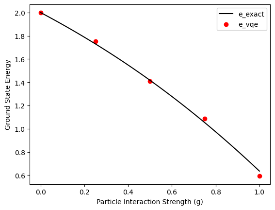
# plot
plt.plot(g_ext_list,e_ext_list,label='e_exact', color="black")
plt.scatter(g_vqe_list,e_vqe_list,label='e_vqe', color="red")
plt.xlabel('Particle Interaction Strength (g)')
plt.ylabel('Ground State Energy')
plt.legend()
plt.show()g = 0.0
e_vqe = 2.0
e_exact = 2.0
g = 0.25
e_vqe = 1.7518310546875
e_exact = 1.7304598458929061
g = 0.5
e_vqe = 1.4091796875
e_exact = 1.416774284351102
g = 0.75
e_vqe = 1.0888671875
e_exact = 1.0527262530578816
g = 1.0
e_vqe = 0.59375
e_exact = 0.6355484735755974