Quantum Error Correction

from qiskit import QuantumCircuit, QuantumRegister, ClassicalRegister
from qiskit_ibm_runtime import QiskitRuntimeService
from qiskit_aer import AerSimulator
from qiskit.visualization import plot_histogram
import numpy as np

Method 1: Repetition Code

q = QuantumRegister(3)
c = ClassicalRegister(3)
qc = QuantumCircuit(q,c)

qc.h(0)

qc.cx(0,1)
qc.cx(0,2)

qc.measure(range(3), range(3))

# Construct a simulator using a noise model from a real backend.
provider = QiskitRuntimeService(channel="ibm_quantum", token="fbc77e68310da5c90990728b892ef5e327787a28a126ad837f8fb88280922284da2784a01e90dc9ccd3be7d48bbe76ca0b8375ac0d3f0f312b1e19da181a18ed")
backend = provider.get_backend("ibm_brisbane")
aersim_backend = AerSimulator.from_backend(backend)
# Perform noisy simulation
results = aersim_backend.run(qc).result().get_counts()
plot_histogram(results)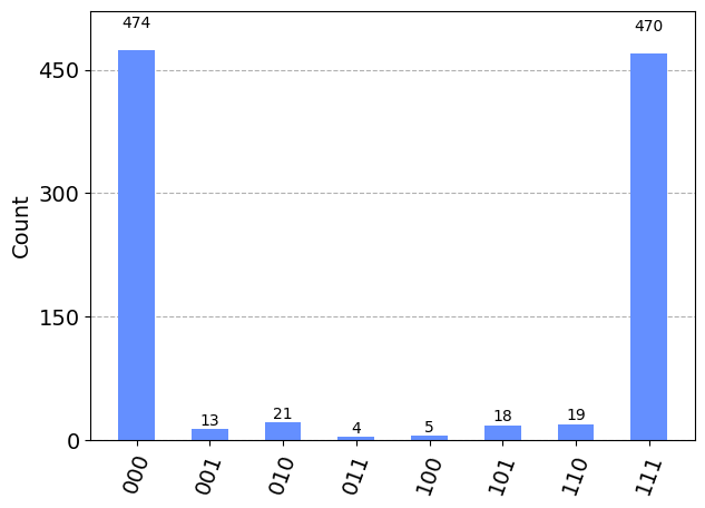

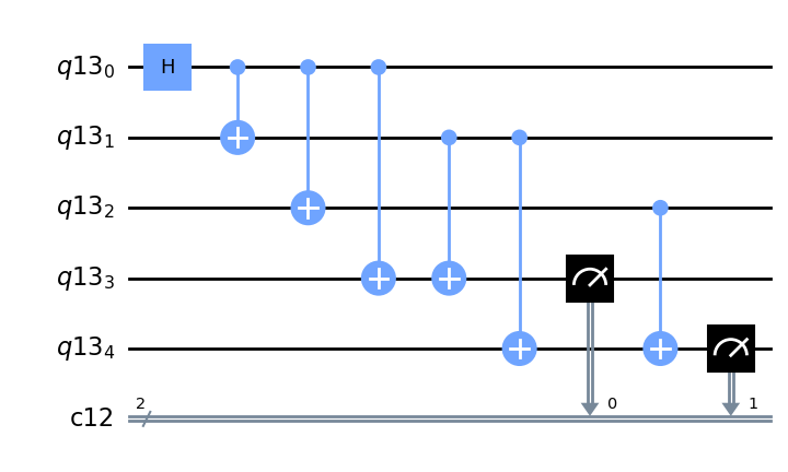
q = QuantumRegister(5)
c = ClassicalRegister(2)
qc = QuantumCircuit(q,c)

qc.h(0)

qc.cx(0,1)
qc.cx(0,2)

qc.cx(0,3)
qc.cx(1,3)

qc.cx(1,4)
qc.cx(2,4)

qc.measure([3,4], range(2))


qc.draw("mpl",style="clifford")

# Construct a simulator using a noise model from a real backend.
#provider = QiskitRuntimeService(channel="ibm_quantum", token="fbc77e68310da5c90990728b892ef5e327787a28a126ad837f8fb88280922284da2784a01e90dc9ccd3be7d48bbe76ca0b8375ac0d3f0f312b1e19da181a18ed")
#backend = provider.get_backend("ibm_brisbane")
#aersim_backend = AerSimulator.from_backend(backend)
# Perform noisy simulation
#results = aersim_backend.run(qc).result().get_counts()
#plot_histogram(results)

q = QuantumRegister(5)
c = ClassicalRegister(2)
qc = QuantumCircuit(q,c)

qc.h(0)

qc.cx(0,1)
qc.cx(0,2)

qc.x(0)

qc.cx(0,3)
qc.cx(1,3)

qc.cx(1,4)
qc.cx(2,4)

qc.measure([3,4], range(2))

# Construct a simulator using a noise model from a real backend.
provider = QiskitRuntimeService(channel="ibm_quantum", token="fbc77e68310da5c90990728b892ef5e327787a28a126ad837f8fb88280922284da2784a01e90dc9ccd3be7d48bbe76ca0b8375ac0d3f0f312b1e19da181a18ed")
backend = provider.get_backend("ibm_brisbane")
aersim_backend = AerSimulator.from_backend(backend)
# Perform noisy simulation
results = aersim_backend.run(qc).result().get_counts()
plot_histogram(results)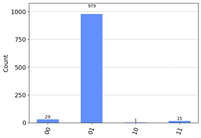

q = QuantumRegister(5)
c = ClassicalRegister(2)
qc = QuantumCircuit(q,c)

qc.h(0)

qc.cx(0,1)
qc.cx(0,2)
qc.h(range(3))

qc.cx(3,0)
qc.cx(3,1)

qc.cx(4,1)
qc.cx(4,2)

qc.h([3,4])

qc.measure([3,4], range(2))

qc.draw("mpl", style="clifford")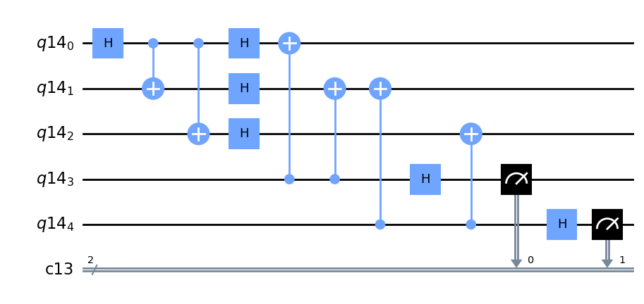

Method 2: Error Mitigation Matrix

q = QuantumRegister(2)
c = ClassicalRegister(2)
qc = QuantumCircuit(q,c)

qc.measure(range(2), range(2))

# Construct a simulator using a noise model from a real backend.
provider = QiskitRuntimeService(channel="ibm_quantum", token="fbc77e68310da5c90990728b892ef5e327787a28a126ad837f8fb88280922284da2784a01e90dc9ccd3be7d48bbe76ca0b8375ac0d3f0f312b1e19da181a18ed")
backend = provider.get_backend("ibm_brisbane")
aersim_backend = AerSimulator.from_backend(backend)
# Perform noisy simulation
results = aersim_backend.run(qc).result().get_counts()
plot_histogram(results)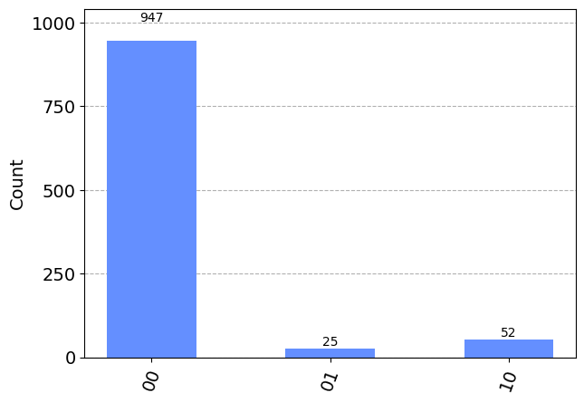

q = QuantumRegister(2)
c = ClassicalRegister(2)
qc = QuantumCircuit(q,c)

qc.x(0)

qc.measure(range(2), range(2))


# Construct a simulator using a noise model from a real backend.
provider = QiskitRuntimeService(channel="ibm_quantum", token="fbc77e68310da5c90990728b892ef5e327787a28a126ad837f8fb88280922284da2784a01e90dc9ccd3be7d48bbe76ca0b8375ac0d3f0f312b1e19da181a18ed")
backend = provider.get_backend("ibm_brisbane")
aersim_backend = AerSimulator.from_backend(backend)
# Perform noisy simulation
results = aersim_backend.run(qc).result().get_counts()
plot_histogram(results)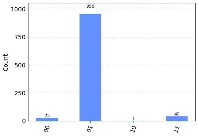

q = QuantumRegister(2)
c = ClassicalRegister(2)
qc = QuantumCircuit(q,c)

qc.x(1)

qc.measure(range(2), range(2))

# Construct a simulator using a noise model from a real backend.
provider = QiskitRuntimeService(channel="ibm_quantum", token="fbc77e68310da5c90990728b892ef5e327787a28a126ad837f8fb88280922284da2784a01e90dc9ccd3be7d48bbe76ca0b8375ac0d3f0f312b1e19da181a18ed")
backend = provider.get_backend("ibm_brisbane")
aersim_backend = AerSimulator.from_backend(backend)
# Perform noisy simulation
results = aersim_backend.run(qc).result().get_counts()
plot_histogram(results)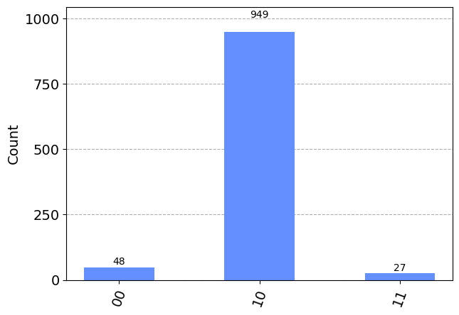

q = QuantumRegister(2)
c = ClassicalRegister(2)
qc = QuantumCircuit(q,c)

qc.x(0)
qc.x(1)

qc.measure(range(2), range(2))

# Construct a simulator using a noise model from a real backend.
provider = QiskitRuntimeService(channel="ibm_quantum", token="fbc77e68310da5c90990728b892ef5e327787a28a126ad837f8fb88280922284da2784a01e90dc9ccd3be7d48bbe76ca0b8375ac0d3f0f312b1e19da181a18ed")
backend = provider.get_backend("ibm_brisbane")
aersim_backend = AerSimulator.from_backend(backend)
# Perform noisy simulation
results = aersim_backend.run(qc).result().get_counts()
plot_histogram(results)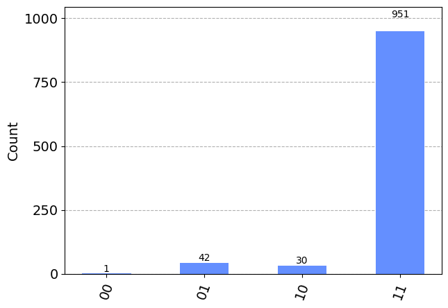

Method 3: Zero Noise Extrapolation

# New installs, mitiq is an error mitigation library we will use for the zero noise extrapolation
# ! pip install ply,mitiq

##############################
##          IMPORT         ##
##############################
# Mitiq imports
from mitiq.benchmarks import generate_ghz_circuit # Creates an example circuit
from mitiq import zne # Zero noise extrapolation

# Qiskit imports
from qiskit import QuantumCircuit
from qiskit import transpile
from qiskit.visualization import plot_histogram

# Aer simulator
from qiskit_aer import AerSimulator

# Fake quantum computer for simulated noise
from qiskit_ibm_runtime.fake_provider import FakeJakartaV2 as FakeJakarta  # Fake (simulated) QPUs
                                                                           # Error based on an older quantum computer

# Number of qubits for the example circuit
n_qubits = 2

# Generate an example circuit which should return either a string of zeros or a string of ones
# equal probability of each return type
#circuit = generate_ghz_circuit(n_qubits=n_qubits, return_type="qiskit")
circuit = QuantumCircuit(2)
circuit.h(range(2))
circuit.cz(0,1)
circuit.h(range(2))
circuit.x(range(2))
circuit.cz(0,1)
circuit.x(range(2))
circuit.h(range(2))
print("GHZ circuit:")
circuit.draw("mpl", style="clifford")

GHZ circuit:

# Number of shots for the simulation
shots = 10 ** 5

# The noiseless backend is the AerSimulator
ideal_backend = AerSimulator()

# Create a copy of the circuit so it is not changed by the first simulation
circuit_to_run = circuit.copy()
# Measure all of the qubits
circuit_to_run.measure_all()

# Compile the circuit into the native gates of the backend
compiled_circuit = transpile(circuit_to_run, ideal_backend)

# Simulate running the circuit on an ideal simulator
ideal_counts = ideal_backend.run(compiled_circuit,shots=shots).result().get_counts()

plot_histogram(ideal_counts)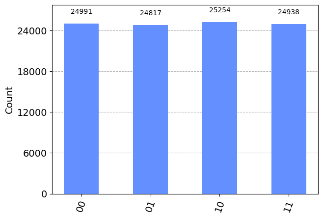

# Use a fake quantum computer modeled off the noise of an older real quantum computer
noisy_backend = FakeJakarta() # QPU emulator

# Compile the circuit into the native gates of the backend
compiled_circuit = transpile(circuit_to_run, noisy_backend)

# Simulate and get the counts
noisy_counts = noisy_backend.run(compiled_circuit, shots=shots).result().get_counts()

# Plot the histogram but make it a bit wider

plot_histogram(noisy_counts,figsize=(15, 5))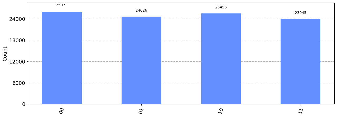

# Calculate the expectation value of an ideal simulation (should be 1)
ideal_expectation_value = (ideal_counts[n_qubits * "1"] ) / shots
print(f"The ideal expectation value is <A> = ", ideal_expectation_value)

# Calculate the expectation value of the noisy simulation
noisy_expectation_value = (noisy_counts[n_qubits * "1"] ) / shots
print(f"The noisy expectation value is <A> = ", noisy_expectation_value)

The ideal expectation value is <A> =  1.0
The noisy expectation value is <A> =  0.92038

# Need to create an execute function which takes a transpile circuit and runs it on the fake quantum computer
# The function needs to return the expectation value, this is used by the mitiq library
def execute(compiled_circuit):
    # Print the depth of the circuit before executing it
    print("Executing a circuit of depth:", compiled_circuit.depth())
    noisy_backend = FakeJakarta()
    noisy_counts = noisy_backend.run(compiled_circuit, shots=shots).result().get_counts()
    noisy_expectation_value = (noisy_counts[n_qubits * "0"] + noisy_counts[n_qubits * "1"]) / shots
    return noisy_expectation_value

# Ensure that this gives similar results to above
print(f"The noisy expectation value is <A> = {execute(compiled_circuit)}")

Executing a circuit of depth: 12
The noisy expectation value is <A> = 0.92472

# Perform zero noise extrapolation, need to pass the transpiled circuit, the execute function
# Can change the options to use different extrapolators and noise methods
zne_value = zne.execute_with_zne(compiled_circuit, executor=execute)
print(f"The error mitigated expectation value is <A> = ", zne_value)

Executing a circuit of depth: 12
Executing a circuit of depth: 26
Executing a circuit of depth: 34
The error mitigated expectation value is <A> =  0.9403999999999985

# Print the error from the ideal expectation value with and without error correction
print(f"Error without ZNE:", abs(ideal_expectation_value - noisy_expectation_value))
print(f"Error with ZNE:", abs(ideal_expectation_value - zne_value))
print("Difference:", abs(ideal_expectation_value - noisy_expectation_value) - abs(ideal_expectation_value - zne_value))

Error without ZNE: 0.07962000000000002
Error with ZNE: 0.05960000000000154
Difference: 0.020019999999998483

Example 2: Variational

import matplotlib.pyplot as plt
import numpy as np

# This time we will use fake noise that we can control the size of, specifically depolarization errors
from qiskit_aer.noise import NoiseModel
from qiskit_aer.noise.errors.standard_errors import depolarizing_error

from mitiq.zne import mitigate_executor
from mitiq.zne.inference import RichardsonFactory

def ansatz(theta):
    """
        Returns a two-qubit circuit for a given variational parameter.
        Inputs:
            theta (a float): The variational parameter.
        Returns:
            circuit (a qiskit circuit): The two-qubit circuit with a fixed gamma.
    """
    circuit = QuantumCircuit(2)
    circuit.rx(theta, 0)
    circuit.cx(0, 1)
    circuit.rx(theta, 1)
    circuit.cx(0, 1)
    circuit.rx(theta, 0)
    
    return circuit

circuit = ansatz(np.pi)
circuit.draw("mpl", style="clifford")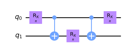

# Define the Hamiltonian of the system
# This will be used to calculate the expectation values
# Because it is z gates then no additional gates need to be 
# added to the circuit before measuring the ansatz
z = np.array([[1,0],[0,-1]])
hamiltonian = np.kron(z, z)

def noiseless_executor(circuit):
    """
        Simulates the execution of a circuit without noise.
        Inputs:
            circuit (a qiskit circuit): The input circuit.
        Returns:
            expectation (a float): The expectation value of the ZZ observable.
    """
    # avoid mutating the input circuit
    circ = circuit.copy()
    # Set up the circuit to save the density matrix
    circ.save_density_matrix()

    # execute experiment without noise, we want the density matrix returned
    simulator = AerSimulator(method="density_matrix")
    
    # Get the density matrix
    rho = simulator.run(circ, shots=1).result().data()["density_matrix"]

    # Compute the expectation value with the Hamiltonian and the density matrix 
    # and return the value
    expectation = np.real(np.trace(rho @ hamiltonian))
    return expectation 
    


# strength of noise channel
noise_level = 0.04

def executor_with_noise(circuit: QuantumCircuit) -> float:
    """
        Simulates the execution of a circuit with depolarizing noise.
        Inputs:
            circuit (a qiskit circuit): The input circuit.
        Returns:
            expectation (a float): The expectation value of the hamiltonian.
    """
    # avoid mutating the input circuit
    circ = circuit.copy()
    circ.save_density_matrix()
    
    # Initialize qiskit noise model. In this case a depolarizing
    # noise model with the same noise strength on all gates, remember that rx is 
    # a 1 qubit gate and cx is a two qubit gate
    noise_model = NoiseModel()
    noise_model.add_all_qubit_quantum_error(depolarizing_error(noise_level, 1), ["rx"])
    noise_model.add_all_qubit_quantum_error(depolarizing_error(noise_level, 2), ["cx"]) 
    
    # execute experiment with depolarizing noise, get the density matrix
    backend = AerSimulator(method="density_matrix", noise_model=noise_model)

    # Transpile the circuit so it can be properly run, optimization level of 0 here so qiskit 
    # does not try to optmize the circuit
    exec_circuit = transpile(circ, backend, basis_gates=noise_model.basis_gates + ["save_density_matrix"], 
                             optimization_level=0)
    
    # Get the density matrix, calculate expectation value and return
    rho = backend.run(exec_circuit, shots=1).result().data()["density_matrix"]

    expectation = np.real(np.trace(rho @ hamiltonian))
    return expectation 

# Perform the noiseless simulation to determine the theta that gives the ground 
# state energy
thetas_noiseless = np.linspace(0, 2 * np.pi, 500)
noiseless_expectations = [noiseless_executor(ansatz(t)) for t in thetas_noiseless]

plt.plot(thetas_noiseless, noiseless_expectations, color="g", linewidth=3, label="Noiseless")
plt.xlabel(r"Ansatz angle $\theta$", fontsize=16)
plt.ylabel(r"$\langle H \rangle(\theta)$", fontsize=16)
plt.legend(fontsize=14)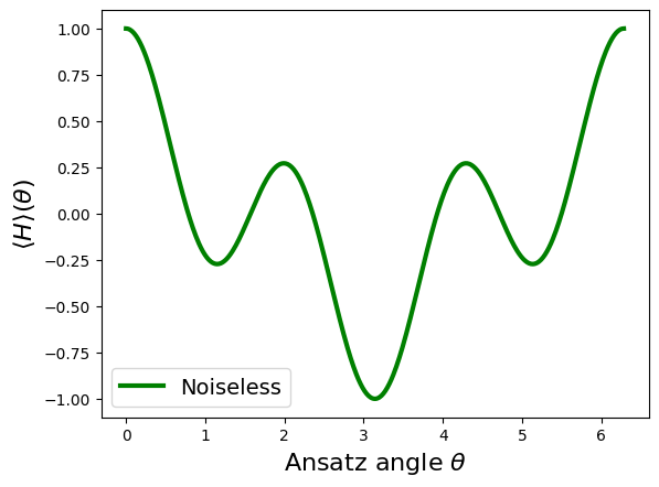

# Perform the simultion with the noisy circuit and compare to noiseless
thetas = np.linspace(0, 2 * np.pi, 50)
expectations = [executor_with_noise(ansatz(g)) for g in thetas]

plt.plot(thetas_noiseless, noiseless_expectations, color="g", linewidth=3, label="Noiseless")
plt.scatter(thetas, expectations, color="r", label="Unmitigated")
plt.xlabel(r"Ansatz angle $\theta$", fontsize=16)
plt.ylabel(r"$\langle H \rangle(\theta)$", fontsize=16)
plt.legend(fontsize=14)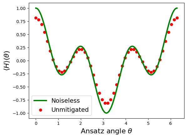

# Richardson extrapolation is a method of extrapolation that can be used for ZNE
# The combination of a Richardson extrapolation with ZNE reduces the time (need less
# points for the extrapolation) and somewhat increases the accuracy
fac = RichardsonFactory(scale_factors=[1, 3, 5])
mitigated_executor = mitigate_executor(executor_with_noise, factory=fac)
mitigated_expectations = [mitigated_executor(ansatz(g)) for g in thetas]

plt.plot(thetas_noiseless, noiseless_expectations, color="g", linewidth=3, label="Noiseless")
plt.scatter(thetas, expectations, color="r", label="Unmitigated")
plt.scatter(thetas, mitigated_expectations, color="b", label="Mitigated")
plt.xlabel(r"Variational angle $\theta$", fontsize=16)
plt.ylabel(r"$\langle H \rangle(\theta)$", fontsize=16)
plt.legend(fontsize=14)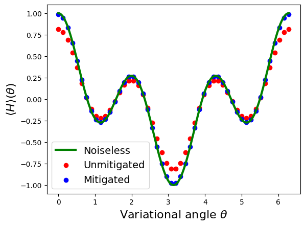

print("Minimum of noiseless landscape:", round(min(noiseless_expectations), 3))
print("Minimum of the noisy landscape:", round(min(expectations), 3))
print("Minimum of the mitigated landscape:", round(min(mitigated_expectations), 3))
print("Theoretical ground state energy:", min(np.linalg.eigvals(hamiltonian)))

Minimum of noiseless landscape: -1.0
Minimum of the noisy landscape: -0.807
Minimum of the mitigated landscape: -0.976
Theoretical ground state energy: -1.0