# Package for building quantum circuits
## ADDED quantum register and classical register to create qubits that map to classical bits
from qiskit import QuantumCircuit, QuantumRegister, ClassicalRegister
# Package for running the quantum code on a simulated quantum computer
from qiskit_aer import AerSimulator
# Package for plotting the results of the quantum code as a histogram
from qiskit.visualization import plot_histogram
## ADDED Numpy for rounding function
import numpy as npSimulating Qubits, Superposition, Entanglement, and Measurement with Qiskit
Imports
Below are the Qiskit imports needed to for this homework. If you need to import any other libraries for your solutions, add the import statements to the below code cell and comment as to why you imported the library or package.
Section 1: Basic Quantum Gates (12 pts.)
This section of the homework will help you a better understanding of how each of the quantum gates affect a single qubit.
- (2 pts.) Create a single qubit and measure its value. Comment on how many times the measurement took place and the results. Visualize your results with a histogram. Are these the expected results?
- (6 pts.) One gate at a time, apply the X, Y, Z, H, and S gates to the single qubit and measure the results. Create a labeled histogram for each experiment to visualize the results. Comment on the results and if they are the expected values.
- (2 pts.) Now focus on just the H gate. Run the code which applies and measures the H gate on the single qubit several times and generate some combined statistics on the results. Comment on the results. Now apply two H gates in series on the qubit and measure, comment, and visualize the results.
q = QuantumRegister(1)
c = ClassicalRegister(1)
qc = QuantumCircuit(q,c)
qc.measure(q,c)
print(qc.draw(output="mpl"))
simulator = AerSimulator()
results = simulator.run(qc).result().get_counts()
plot_histogram(results)

## 1,024 measurements take place when running the Aer simulator with the default settings
Figure(203.885x200.667)
q = QuantumRegister(1)
c = ClassicalRegister(1)
qc = QuantumCircuit(q,c)
qc.x(0)
qc.measure(q,c)
print(qc.draw(output="mpl"))
simulator = AerSimulator()
results = simulator.run(qc).result().get_counts()
plot_histogram(results)
Figure(287.496x200.667)
q = QuantumRegister(1)
c = ClassicalRegister(1)
qc = QuantumCircuit(q,c)
qc.y(0)
qc.measure(q,c)
print(qc.draw(output="mpl"))
simulator = AerSimulator()
results = simulator.run(qc).result().get_counts()
plot_histogram(results)
Figure(287.496x200.667)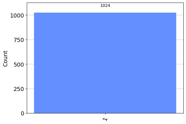
q = QuantumRegister(1)
c = ClassicalRegister(1)
qc = QuantumCircuit(q,c)
qc.z(0)
qc.measure(q,c)
print(qc.draw(output="mpl"))
simulator = AerSimulator()
results = simulator.run(qc).result().get_counts()
plot_histogram(results)
Figure(287.496x200.667)
q = QuantumRegister(1)
c = ClassicalRegister(1)
qc = QuantumCircuit(q,c)
qc.h(0)
qc.measure(q,c)
print(qc.draw(output="mpl"))
simulator = AerSimulator()
results = simulator.run(qc).result().get_counts()
plot_histogram(results)
Figure(287.294x200.667)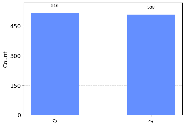
q = QuantumRegister(1)
c = ClassicalRegister(1)
qc = QuantumCircuit(q,c)
qc.s(0)
qc.measure(q,c)
print(qc.draw(output="mpl"))
simulator = AerSimulator()
results = simulator.run(qc).result().get_counts()
plot_histogram(results)
Figure(287.496x200.667)
count = 5000
zero_results = 0
one_results = 0
for i in range(count):
    q = QuantumRegister(1)
    c = ClassicalRegister(1)
    qc = QuantumCircuit(q,c)
    qc.h(0)
    qc.measure(q,c)
    simulator = AerSimulator()
    results = simulator.run(qc).result().get_counts()
    zero_results += results["0"]
    one_results += results["1"]

tot_results = zero_results + one_results
print("Number of 0/up states:", zero_results)
print("Number of 1/down states:", one_results)
print("Total number of states:", tot_results)
print("Percent of 0/up:", np.round(zero_results/tot_results*100, 2))
print("Percent of 1/down:", np.round(one_results/tot_results*100,2))
Number of 0/up states: 2559256
Number of 1/down states: 2560744
Total number of states: 5120000
Percent of 0/up: 49.99
Percent of 1/down: 50.01count = 1000
zero_results = 0
one_results = 0
for i in range(count):
q = QuantumRegister(1)
c = ClassicalRegister(1)
qc = QuantumCircuit(q,c)
qc.h(0)
qc.h(0)
qc.measure(q,c)
simulator = AerSimulator()
results = simulator.run(qc).result().get_counts()
zero_results += results["0"]
tot_results = zero_results + one_results
print("Number of 0/up states:", zero_results)
print("Number of 1/down states:", one_results)
print("Total number of states:", tot_results)
print("Percent of 0/up:", np.round(zero_results/tot_results*100, 2))
print("Percent of 1/down:", np.round(one_results/tot_results*100,2))Number of 0/up states: 1024000
Number of 1/down states: 0
Total number of states: 1024000
Percent of 0/up: 100.0
Percent of 1/down: 0.0Section 2: Two Qubit Superposition (7 pts.)
This section of the homework will test if two qubits are entangled with each other.
- (1 pt.) Create the two qubit state \(|00\rangle\). Measure the results and visualize with a histogram to prove that you have created the correct state.
- (3 pts.) Apply the Hadamard gate to the first qubit and the apply the CNOT gate with the first qubit as the control and the second qubit as the target. What superposition of states have you created (don’t forget the normlization constant)?
- (3pts.) How can you show that you have properly entangled your two qubits? Design and carry out an experiment to show this.
q = QuantumRegister(2)
c = ClassicalRegister(2)
qc = QuantumCircuit(q,c)
qc.measure(q,c)
print(qc.draw(output="mpl"))
simulator = AerSimulator()
results = simulator.run(qc).result().get_counts()
plot_histogram(results)
Figure(360.822x284.278)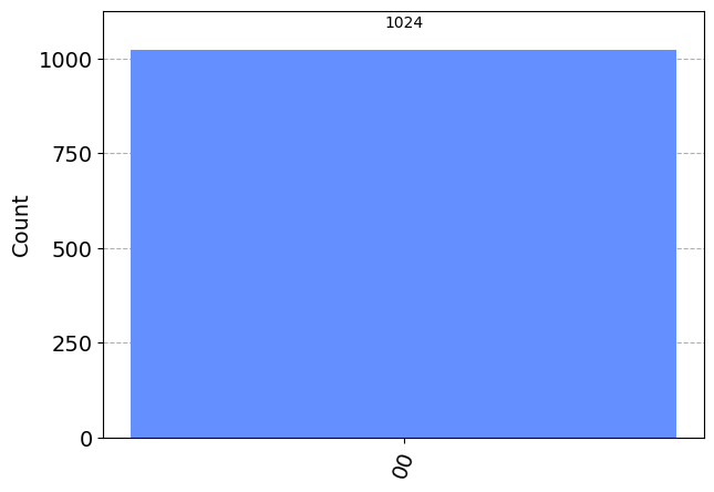
q = QuantumRegister(2)
c = ClassicalRegister(2)
qc = QuantumCircuit(q,c)
qc.h(0)
qc.cx(0,1)
qc.measure(q,c)
print(qc.draw(output="mpl"))
simulator = AerSimulator()
results = simulator.run(qc).result().get_counts()
plot_histogram(results)
Figure(527.641x284.278)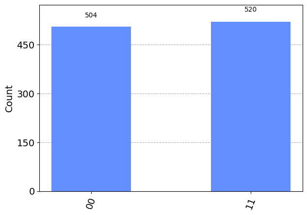
q = QuantumRegister(2)
c = ClassicalRegister(2)
qc = QuantumCircuit(q,c)
qc.h(0)
qc.cx(0,1)
qc.measure(q,c)
print(qc.draw(output="mpl"))
simulator = AerSimulator()
results = simulator.run(qc, shots=10000).result().get_counts()
plot_histogram(results)
Figure(528.045x284.278)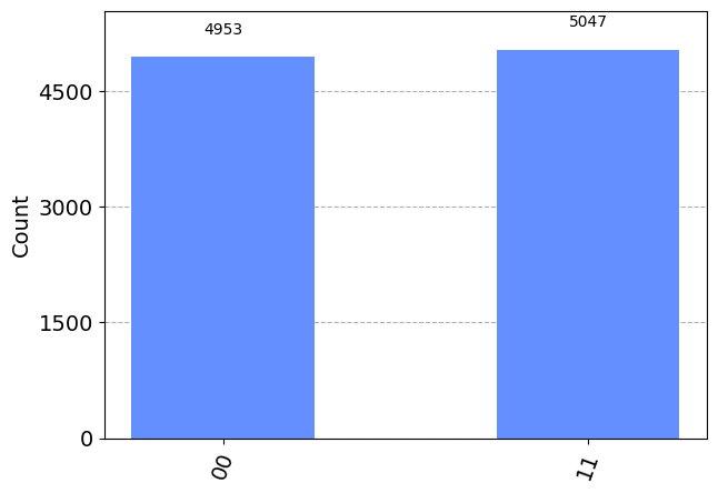
Section 3: Bell States (13 pts.)
The state you made in Section 2 is one of four Bell states. The Bell states are: \[\frac{1}{\sqrt{2}}(|00\rangle + |11\rangle)\] \[\frac{1}{\sqrt{2}}(|00\rangle - |11\rangle)\] \[\frac{1}{\sqrt{2}}(|01\rangle + |10\rangle)\] \[\frac{1}{\sqrt{2}}(|01\rangle 1 |10\rangle)\]
- (3 pts.) Which Bell state did you create in Section 2? Explain your answer.
In Section 2 we made the \(\frac{1}{\sqrt{2}}(|00\rangle + |11\rangle)\) since we only measured the states \(|00\rangle\) and \(|11\rangle\) and there was no negative phase.
- (10 pts.) Create the Bell state \(\frac{1}{\sqrt{2}}(|01\rangle + |10\rangle)\). Prove that you have properly entangled the qubits.
q = QuantumRegister(2)
c = ClassicalRegister(2)
qc = QuantumCircuit(q,c)
qc.h(0)
qc.x(1)
qc.cx(0,1)
qc.measure(q,c)
print(qc.draw(output="mpl"))
simulator = AerSimulator()
results = simulator.run(qc, shots=10000).result().get_counts()
plot_histogram(results)
Figure(528.045x284.278)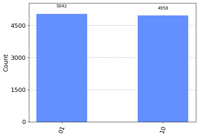
Section 4: Three Qubit Entanglement (20 pts.)
This section will have you explore creating quantum circuits with three entangled qubits. 1. (2 pts.) Create the three qubit state \(|000\rangle\). Prove that you have made this state. 2. (15 pts.) Apply any gates to this three qubit state such that you get two or more possible states upon measurement. What state (including normalization constants) have you created? Construct a theoretical answer and then test to see if it is true. 3. (3 pts.) Prove that you have properly entangled your three qubits.
q = QuantumRegister(3)
c = ClassicalRegister(3)
qc = QuantumCircuit(q,c)
qc.measure(q,c)
print(qc.draw(output="mpl"))
simulator = AerSimulator()
results = simulator.run(qc).result().get_counts()
plot_histogram(results)
Figure(444.636x367.889)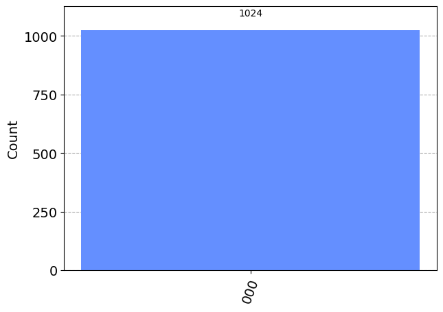
q = QuantumRegister(3)
c = ClassicalRegister(3)
qc = QuantumCircuit(q,c)
qc.measure(q,c)
qc.x(1)
qc.h(0)
qc.cswap(0,1,2)
print(qc.draw(output="mpl"))
simulator = AerSimulator()
results = simulator.run(qc).result().get_counts()
plot_histogram(results)
Figure(528.045x367.889)