Quantum Mechanics Crash Course (Part 1): Concepts and Statistics

Author: Julie Butler

Date Created: July 6, 2024

Last Modified: August 19, 2024

Back to course page.

What Makes Up Matter?

All matter is made up of atoms and molecules (and all molecules are made up of atoms). Atoms are not indivisible; they can be broken up into smaller components. An atom is made up of a dense, positively charged nucleus surrounded by small, negatively charged electrons. Most of the mass of the atom is contained in the nucleus but most of the volume an atom occupies is empty space; the electrons “orbit” the nucleus at very fast speeds. A force called the Coulomb force holds the electrons to the nucleus because of their charges (opposite charges attract, same charges repel).

Electrons, as far as we know, can not be further divided (they are said to be elementary particles in the standard model of physics). The nucleus, however, can be divided into particles called protons and neutrons. A proton and a neutron have a similar mass, but the protons are positively charged and the neutrons are negatively charged. The magnitude of charge for a proton and an electron are the same (i.e. the number is the same) but the sign of the charge is different. The positively charged protons are why the nucleus is positively charged and attracts the electrons needed to form an atom. However, the positively charged protons want to repel each other (same charges repel) but there is another force, which only exist in the nucleus, which resists this repulsion and holds the protons and neutrons together. This is called the strong force. Note that neutrons and protons can be further divided into even smaller particles called quarks, but we will not study quarks in this course (if interested, quarks are covered in particle physics courses).

The number of protons in the nucleus defines the type of atom, i.e., what element it belongs to. For example, every atom which has six protons in its nucleus is carbon. An atom will typically have no net charge (the net charge is calculated by adding up the individual charges of every particle), meaning that the number of electrons in the atom is the same as the number of protons. Note this is not always true: electrons can be added or removed from a atom, creating ions (though this veers into the field of chemistry instead of quantum mechanics). The number of neutrons in the nucleus does not define the type of element, and is (typically) not the same as the number of protons. Two atoms which contain the same number of protons (and thus are the same element) but have different numbers of neutrons are called isotopes. The isotope of an element determines how stable it is (nuclei that do not have specific amounts of protons and neutrons are unstable and will eventually decay into smaller nuclei).

Molecules, atoms, nuclei, electrons, protons, neutrons, and other small particles do not obey the same rules of physics that macroscopic objects obey (this type of physics is called classical physics). Instead, quantum mechanics describes the behavior of things so small we cannot see them. It implements a new set of rules that these systems obey instead of classical physics. Quantum mechanical systems (a system is an object or objects we are studying) are not deterministic, meaning we can not know the exact result of measuring the position, speed, energy, etc. of a system. Quantum mechanical systems are instead probabilistic; the results of experiments are statistically random, but still describable!

Light and Photons

In classical physics, we think of light as being a wave, specifically electromagnetic radiation. In fact, in many experiments such as the double-slit experiment, light does behave as a wave. However, there are some experiments which can be performed using light that produce results that cannot be explained if light is only a wave. For example, there is an experiment called the photoelectric effect where light is directed onto an exposed wire. If the correct wavelengths of light (higher in energy) are used then the light can give the electrons in the metal enough energy to break free and produce a current. However, if lower energy wavelengths are used then no matter how bright the light is (how intense the light is) no electrons will break free and produce a current. The results of this experiment and its interpretation, gave Einstein his Nobel Prize. The only way to explain the photoelectric effect is if we consider light to not be a light but to be made up of tiny, massless particles called photons. In fact, light has both particle and wave properties, resulting in something called a wave-particle duality.

Wave-Particle Duality

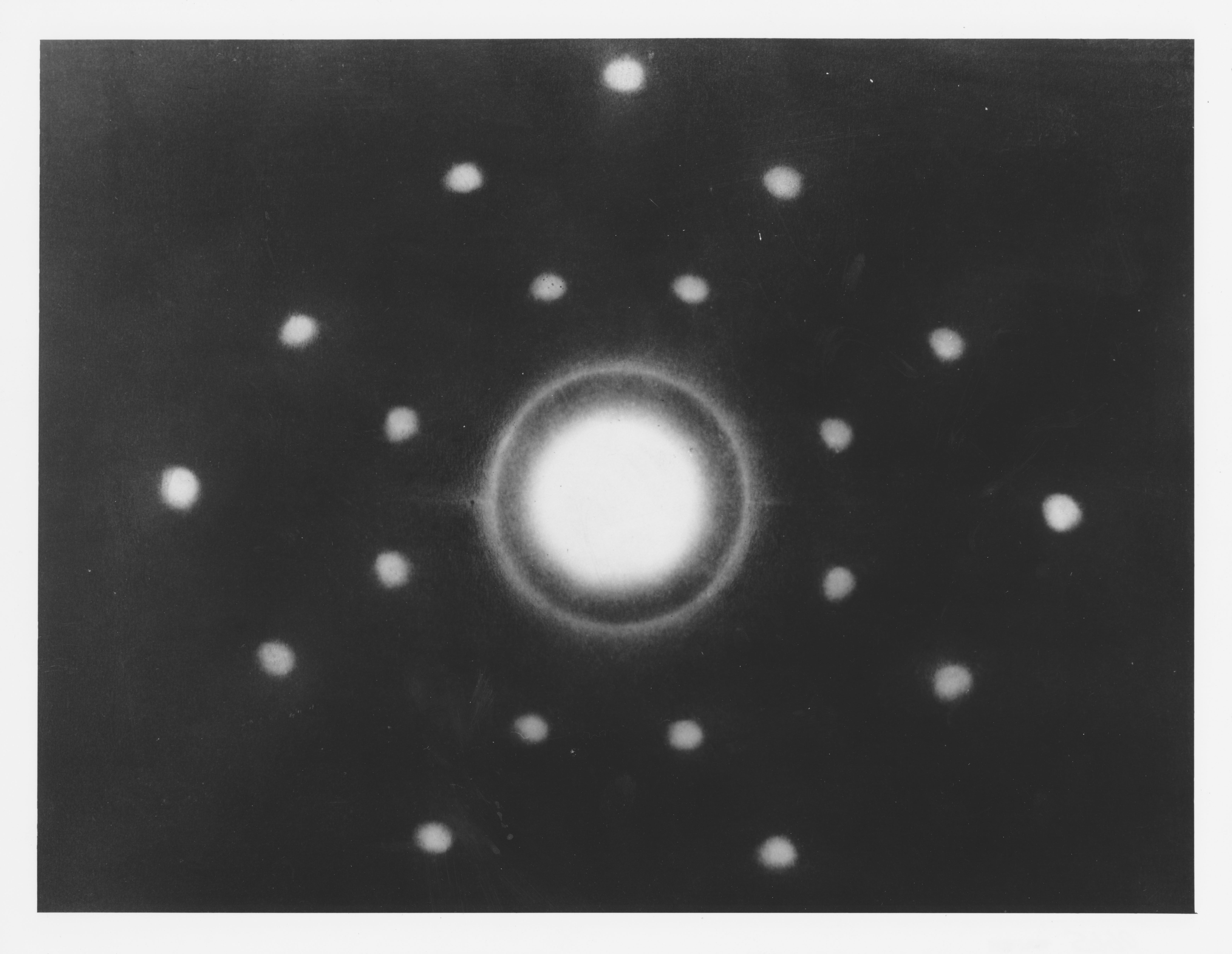
We say that light has a wave-particle duality because it displays properties of both waves and particles, depending on the experiment being performed. However, this duality is not limited to light. Particles so small that they require quantum mechanics to describe their motion (electrons, protons, neutrons, etc.) also exhibit wave light qualities under certain experiments. For example, compare the images from a neutron scattering experiment to those from a double-slit experiment. Thus, small particles also have a wave-particle duality and we utilize this feature a lot in quantum mechanics. We describe particles with a wavefunction, we can talk about the average position of a particle but not its exact position (what is the location of a wave?), and many other features that we will discuss in the coming weeks.

Interlude: Probability and Statistics

Since quantum mechanics is a probabilistic system, we need to have a good background in probability and statistics before we can begin developing the relevant mathematics. First, we need to discuss the difference between discrete and continuous variables. Discrete variables describe data that can only be certain values. Flipping a coin can only result in “heads” or “tails”. The odometer on a car only reads whole miles. The money in a bank account increases or decreases in increments of one cent. Continuous variables, on the other hand, can be any number in a given range. The temperature of a room can be any number, a car can go down the road at any speed.

We call the outcome of a measurement an event. In the case of flipping a coin, the possible events are “heads” or “tails”. We can represent a heads as a 0 and a tails as a 1. Then, the number of times flipping a coin and getting heads is $N(0)$, and the number of times of getting tails is $N(1)$. The total number of events is the sum of the number of times a given outcome occurs. So the total number can be defined as:

$$N=\sum _{j=0}^{\mathrm{\infty }}N(j),$$

where j are the possible events that come from taking a measurement of a system and N(j) is the number of times event j occurred.

Discrete Variables Example

Consider a room containing 14 people who have the following ages:

• one person aged 14
• one person aged 15
• three people aged 16
• two people aged 22
• two people aged 24
• five people aged 25

The way we typically use age, it is a discrete variable, only taking whole numbers.

We can then define the number of people of a certain age as:

• N(14) = 1
• N(15) = 1
• N(16) = 3
• N(22) = 2
• N(24) = 2
• N(25) = 5

Probability

Discrete Variables

With discrete variables, the probability of event j happening, $P(j)$, is simply the number of times event j happened, $N(j)$, divided by the total number of events, $N$.

$$P(j)=\frac{N(j)}{N}$$

Note that the total probability of any possible event occurring must be 1 (there is a 100% chance that measuring the outcome results in one of the possible events) so $\sum _{j=0}^{\mathrm{\infty }}P(j)=0$.

Continuous Variables

For continuous variables, since there is an infinite number of possible events, we need to consider a different formulation. Instead of the probability of a certain event occurring, we will instead discuss the probability of the result of a measuring being between a and b:

$$P_{ab}={\int }_a^b\rho (x)dx,$$

where we have defined $\rho (x)$ to be the probability density. You can interpret this as a function which returns the probability of event $x$ occurring. We will give a more physical meaning to probability densities in later lectures. For now, the higher the probability density at a given input, the more likely that event is to occur. Note that since all probabilities must add to 1, we have to impose the condition that ${\int }_{-\mathrm{\infty }}^{\mathrm{\infty }}\rho (x)dx=1$.

Discrete Variables Examples

Let’s remember our data set from the previous example:

• N(14) = 1
• N(15) = 1
• N(16) = 3
• N(22) = 2
• N(24) = 2
• N(25) = 5

We can calculate to probabilities of each of these events occurring using $P(j)=\frac{N(j)}{N}$, where N = 14:

• P(14) = 1/14 $\approx$ 0.071
• P(15) = 1/14 $\approx$ 0.071
• P(16) = 3/14 $\approx$ 0.214
• P(22) = 2/14 $\approx$ 0.142
• P(24) = 2/14 $\approx$ 0.142
• P(25) = 2/14 $\approx$ 0.357

Note that $\frac{1}{14}+\frac{1}{14}+\frac{3}{14}+\frac{2}{14}+\frac{2}{14}+\frac{5}{14}=\frac{14}{14}=1$; the probability of choosing a person from the room who is age 14, 15, 16, 22, 24, or 25 is 100%. The most probable age of a randomly selected person is 25 since this age has the highest probability.

Average (Mean) or Expectation Value

Since quantum mechanics is a probabilistic system, we will typically refer to the average measurement instead of an exact measurement. Note that both average and mean have the same definition: the most likely outcome of a measurement. In the context of quantum mechanics, we will typically use the phrase expectation value instead of average but they have the same meaning.

We will denote the expectation value for a quantity j as $⟨j⟩$. For discrete variables we will define the expectation values as:

$$⟨j⟩=\frac{\sum jN(j)}{N}=\sum _{j=0}^{\mathrm{\infty }}jP(j),$$

and for continuous variables as:

$$⟨x⟩={\int }_{-\mathrm{\infty }}^{\mathrm{\infty }}x\rho (x)dx$$

Discrete Variables Example

What is the expectation value (average) for the age of all people in the room?

$$⟨j⟩=14(\frac{1}{14})+15(\frac{1}{14})+16(\frac{3}{14})+22(\frac{2}{14})+24(\frac{2}{14})+25(\frac{5}{14})$$ $$⟨j⟩=21$$

The interpretation of this result is that if you randomly select a single person from this room over and over, eventually the average age of all of your picks will be 21. Note that 21 is not a possible measurement, however. There is a difference between expectation value and measurement.

Other Expectation Values

We can also calculate the expectation value of other quantities which depend on your data. Simply replace j or x in the previous equations with a function of j or x. So, for discrete data we have:

$$⟨f(j)⟩=\sum _{j=0}^{\mathrm{\infty }}f(j)P(j),$$

and for continuous variables we have:

$$⟨f(x)⟩={\int }_{-\mathrm{\infty }}^{\mathrm{\infty }}f(x)\rho (x)dx.$$

Discrete Variables Example

Let’s assume that there is a simple formula that relates a person’s age, a, to the costs of their health insurance, I:

$$I=5a+7$$

For the room of people we have, the expectation value for their health insurance cost is:

$$⟨I⟩=(5(14)+7)(\frac{1}{14})+(5(15)+7)(\frac{1}{14})+(5(16)+7)(\frac{3}{14})+(5(22)+7)(\frac{2}{14})+(5(24)+7)(\frac{2}{14})+(5(25)+7)(\frac{5}{14})$$

$$⟨I⟩=112.0$$

Standard Deviation

The final statistical calculation we need to look at is the standard deviation, which measures the spread of the data. A large standard deviation indicates that the data is very spread out while a small standard deviation indicates that the data is clustered around the average value. We will denote the standard deviation is $\sigma$, occasionally with a subscript to denote the quantity it belongs to. The equation is the same for either continuous or discrete variables: $$\sigma =\sqrt{⟨x^2⟩-⟨x{⟩}^2},$$ where $⟨x{⟩}^2$ is the expectation value squared for the data set and $⟨x^2⟩$ is the expecation value of the squared data.

Discrete Variables Example

The standard deviation of our ages data set can be calculated as follows. We found earlier that $⟨j⟩=21$, so now we need to find $⟨j^2⟩$.

$$⟨j^2⟩={14}^2(\frac{1}{14})+{15}^2(\frac{1}{14})+{16}^2(\frac{3}{14})+{22}^2(\frac{2}{14})+{24}^2(\frac{2}{24})+{25}^2(\frac{5}{14})$$

$$⟨j^2⟩\approx 459.57$$

Now we can calculate the standard deviation:

$$\sigma =\sqrt{⟨j^2⟩-⟨j{⟩}^2}=\sqrt{459.57-{21}^2}\approx 4.30$$

This tells us that 67% of people in the room are within 4.30 years of our average age. This also tells us that there is a wide variety of ages in the room as 4.30 years is quite large considering that there is only 9 years between the oldest and youngest people in the room.

Events and Likelihoods

Now that we have the statistics defined, let’s work on some new notation. Let’s consider the results of flipping a quarter, Q. There is a 50% chance of getting heads (H) and a 50% chance of getting tails (T). We will represent the event of flipping a quarter as $|Q⟩$ as the sum of its possible outcomes, $|H⟩$ and $|T⟩$. Hint: the bra-ket notation should give you a hint for what we will do on Monday. Thus, we can say that the outcome from flipping a quarter is:

$$|Q⟩=\sqrt{\frac{1}{2}}|H⟩+\sqrt{\frac{1}{2}}|T⟩$$

Note that the coefficients on $|H⟩$ and $|T⟩$ are not random, they have an important meaning. If you take the modulus squared of the coefficient of $|H⟩$ you get the probability of the event $|H⟩$ happening: $|\sqrt{\frac{1}{2}}{|}^2=0.5=50\mathrm{\%}|$. The same is true for $|T⟩$.

Also note that if we sum the modulus squared values of the coefficients (if we sum the probabilities) we get 1: $|\sqrt{\frac{1}{2}}{|}^2+|\sqrt{\frac{1}{2}}{|}^2=1$. The interpretation is that there is a probability of 1 (100%) that when you measure the outcome of a quarter flip you get one of the possible outcomes.

Wavefunction

In the last section we created a representation for the events that occur when flipping a quarter. We use this same idea when writing an equation to represent a quantum mechanical state, called a wavefunction, typically represented as $|\psi ⟩$ (with a variety of Greek letters in addition to $\psi$). A wavefunction tells you everything that can be known about a quantum mechanical state. You extract the information about the state through mathematical operations like expectation values and standard deviations (more of this on Monday).

Spin

All particles have certain properties that define what type of particle they are. For example, all particles have mass, which determines how a particle interacts with the gravitational force, and all particles have charge, which determines how a particle ineteracts with the electric force. A proton and neutron have very similar masses, but a protons has a positive charge and a neutron has no charge. An electron has a negative charge and a proton has a positive charge. However, even particles of the same type, such as electrons, which have the same mass and the same charge, can interact with the magnetic force differently because they have different values of spin.

Spin is a property that in intrinsic to all particles, but it is not related to the particle “spinning” in space. Rather, like mass and charge, it is a property that can be determined by observing how a particle interacts with various fields (graviational for mass, electric for charge, and magentic for spin). Spin occurs in three directions, known as x, y, and z (Cartesian space). Spin can have two values in each direction: $$1. In this class we will primarily be focusing on spin in the z-direction, where a value of +1 is referred to as spin up and a spin value of -1 is referred to as spin down. We can think of this spin as an arrow on the Bloch sphere.

Bloch Sphere

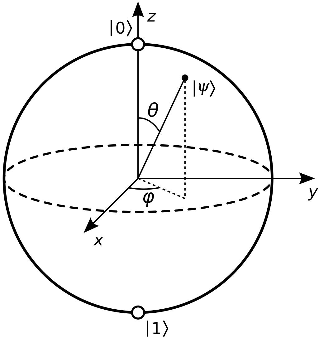
This sphere should look familiar as we used to on Monday to discuss a qubit. In fact, we will be considering the z-direction spin of a particle quite often in this course as it is one of the most common ways to define the two states of a qubit: spin up represents the 0 state of the qubit and spin down represents the 1 state. Note that this is not the only way to define the two states of a qubit with a physical system, and we will learn about other models later in this course.

Note: properties of a particle that can have different values are referred to as degrees of freedom.

Spin Up and Spin Down

In this course we will see several different ways to represent the spin of a particle, but we will start by using an intuitive symbolism: spin-up is represented as $|\uparrow ⟩$ and spin-down is represented as $|\downarrow ⟩$. Note the bracket notation should give you a hint that we will eventually be considering these quantities as vectors. As we learned on Monday, the difference in a classical computer and a quantum computer is that a qubit in a quantum computer is not in just one of the two states, but it can be in a superposition of both the 0 and the 1 state at the same time. Thus, we need to develop a formalism which will allows us to write a state that is somehow simultaneously in the spin-up and the spin-down states. Let’s start with a state, $|\psi ⟩$, written as follows:

$$|\psi ⟩=\frac{4}{5}|\uparrow ⟩-\frac{3i}{5}|\downarrow ⟩$$

Superposition

If a quantum state can be in two or more different states at the same time, then we say that the quantum state is in a superposition of different states. A qubit is typically referred to as being in a superposition of the spin-up, $|\uparrow ⟩$, and the spin-down, $|\downarrow ⟩$, states. Let’s bring back the qubit state we were looking at in the previous section: $$|\psi ⟩=\frac{4}{5}|\uparrow ⟩-\frac{3i}{5}|\downarrow ⟩$$

Measurement

A problem occurs in quantum mechanics when we wish to study a system and measure its properties. Any interaction strong enough to measure a quantum mechanical system is strong enough to change it. This means that if we have a sustem which is in a superposition of states, when we measure the system we force it to collapse to only one state (it will no longer in in a superposition). We say that the first measurement a system receives prepares it for additional measurements.

Let’s consider an electron which can be either spin up or spin down. Before its first measurement, it is in the following superposition:

$$|\psi ⟩=\frac{4}{5}|\uparrow ⟩-\frac{3i}{5}|\downarrow ⟩$$

When the above state is measured, it is forced to collapse to either $|\uparrow ⟩$ or $|\downarrow ⟩$; it will no longer be in a superposition of both states. The probability it will collapse into $|\uparrow ⟩$ is $|\frac{4}{5}{|}^2=\frac{16}{25}$ and the probability that it will collapse into $|\downarrow ⟩$ is $|\frac{3i}{5}{|}^2=\frac{9}{25}$. Note that $P(|\uparrow ⟩)+P(|\downarrow ⟩)=\frac{16}{25}+\frac{9}{25}=\frac{25}{25}=1$ (the probability that when the state is measure it collapses into one of the states that make it up is 100%).

Operators and Observables

When we measure a quantum mechanical state, we say we are applying an operator to the state and the result of this is the measurement of an observable. For example, the momentum operator is applied to a quantum state and the returned observable is the momentum of the state. Only certain states and observables are possible for a given operator, but we will go into more detail on this Monday.

Example: Superposition, Measurement, and State Preparation

An operator $\hat{A}$, representing observable A, has two normalized states ${\psi }_1$ and ${\psi }_2$, with values $a_1$ and $a_2$, respectively. Operator $\hat{B}$, representing observable B, has two normalized states ${\psi }_1$ and ${\psi }_2$ with values $b_1$ and $b_2$. The states are related by

$${\psi }_1=(3{\varphi }_1+4{\varphi }_2)/5{\psi }_2=(4{\varphi }_1-3{\varphi }_2)/5$$

• Observable A is measured, and the value $a_1$ is obtained. What is the state of the system immediately after this measurement?
  • If $a_1$ is obtained on the measurement of the observable A, then this means that the state has collapsed into the wavefunction which will give $a_1$. Thus, immediately after this measurement the system is in state ${\psi }_1$. This is the only way in which $a_1$ could have been measured.
• If B is now measured, what are the possible results, and what are their probabilities?
  • Since we are in the state ${\psi }_1$, we need to look at the wavfunction ${\psi }_1=(3{\varphi }_1+4{\varphi }_2)/5$ to determine the possible outcomes of measuring the observable B and the probabilities of each outcome. ${\psi }_1$ can be written as a superposition of the two possible outcomes of measuring observable B, ${\varphi }_1$ and ${\varphi }_2$. Thus both outcomes are possible and we can determine the probabilities by looking at the coefficients. Since the coefficient on ${\varphi }_1$ is $\frac{3}{5}$ the probability of obtaining ${\varphi }_1$ on the measurement of B when the state is already in ${\psi }_1$ is $|\frac{3}{5}{|}^2=\frac{9}{25}$. Likewise, since the coefficient on ${\varphi }_2$ is $\frac{4}{5}$ the probability of obtaining ${\varphi }_2$ on the measurement of B when the state is already in ${\psi }_1$ is $|\frac{4}{5}{|}^2=\frac{16}{25}$. If the state collapses into ${\varphi }_1$ then the resulting measurement is $b_1$ (with a probability of $\frac{9}{25}$) and if the state collapses into ${\varphi }_2$ then the resulting measurement is $b_2$ (with a probability of $\frac{16}{25}$). Note that $P(b_1)+P(b_2)=\frac{9}{25}+\frac{16}{25}=\frac{25}{25}=1$.

Entanglement

In the previous example, the states of $\hat{A}$ and the states of $\hat{B}$ are entangled. This means that what happens to one set of states changes what happens to the other set of states. When we initially measured $\hat{A}$ and collapsed to the state ${\psi }_1$, we changed the probabilities of getting ${\varphi }_1$ and ${\varphi }_2$ on the measurement of $\hat{B}$ compared to if the state had collapsed into ${\psi }_2$ on the measurement of $\hat{A}$ instead.

Most of the quantum mechanical states we will be dealing with in this class are entangled. In a quantum computer which has more than one qubit, all of the qubits represented quantum mechanical states which are entangled with each other.

Uncertainty

Uncertainty is a big problem in quantum mechanics because it controls what properties of a system we can measure at the same time. Certain pairs of properties can be measured simultaneously on a single quantum mechanical system, but only within a set uncertainty. For example, you can measure the position and momentum of a system simultaneously, but the product of the uncertainties on the measurements (${\sigma }_x{\sigma }_p$) must be greater than $\hslash /2$, where $\hslash$ is a constant known as Planck’s reduced constant. In quantum computing, when we want to measure various attributes of a quantum system, we need to be careful that we are not measuring observables simultaneously if they have an uncertainty principle.

Energy

The energy of a system is an important quantity in quantum mechanics because it allows us to determine a system’s potential to do … something. We measure the energy of macroscopic objects as well, and we consider the energy we measure of these large object to be a continuous variable. However, this is not necessarily true for quantum mechanical systems. For these systems energy is quantized, meaning it can only have certain set values.

Spin is another example of a quantized observable, where the only possible results of measuring the spin of a particle are spin up (+1) or spin down (-1). No other result is possible.

References and Resources

• Quantum Mechanics: The Theoretical Minimum. Leonard Susskind.
• Introduction to Quantum Mechanics. David J. Griffiths and Darrell F. Schroeter. 3rd. ed.
• If You Don’t Understand Quantum Physics, Try This! (Video)