# Import Numpy for linear algebra
import numpy as np

# Define the two possible states of a single qubit
up = np.array([1,0])
down = np.array([0,1])

# Define a down qubit
qubit = down
print("Example Qubit:")
print(qubit)
Example Qubit:
[0 1]We will start by learning how to handle a quantum computer containing only one qubit. This single qubit computer does not have many real-world applications but it does allow us to learn about quantum gates and the Qiskit library without too many complications.
A one-qubit system can be in two different states. We will represent these with the following two basis vectors we have seen several times at this point.
\[|\uparrow\rangle = |0\rangle = \begin{bmatrix}1\\0\end{bmatrix} \quad |\downarrow\rangle = |1\rangle = \begin{bmatrix} 0\\1\end{bmatrix}\]
We will go into physical implementations of quantum computers near the end of the course, but for now, let’s consider the qubit to be an electron and we are measuring and altering the spin in the z-direction (spin-up will be the \(|\uparrow\rangle\) state and \(|\downarrow\rangle\) will be the spin-down state). If you want to know a bit more about actual implementations of a quantum computer check out this video from Domain of Science. Scientists are testing many different implementations for quantum computers with the only restriction is the system needs to have two states that it can be easily manipulated to change between (we need two states to represent the two values of a single qubit).
The following code imports the Numpy library, defines the two qubit states as Numpy arrays of length 2, and then creates a qubit in the down state.
# Import Numpy for linear algebra
import numpy as np
# Define the two possible states of a single qubit
up = np.array([1,0])
down = np.array([0,1])
# Define a down qubit
qubit = down
print("Example Qubit:")
print(qubit)Example Qubit:
[0 1]For a single qubit, a gate is a 2x2 matrix that manipulates a qubit. This might mean changing it from \(|\uparrow\rangle\) to \(|\downarrow\rangle\) (or vice versa), creating a superposition of the two states, or adding phase factor (a sign change) to the qubit.
A gate is an matrix like an operator BUT a gate does not collapse a superposition becuase there is no measurement being performed. This means that if a superposition of states enters the gate, the same superposition of states will leave the gate.
There are some constraints on what types of matrices can be quantum gates: the matrices must be unitary. This means that for a quatum gate U, if you multiply iy by its adjoint you will get the identity matrix (\(U^\dagger U\) = I). Note that this is required because quantum gates must be reversible: for every quantum gate there exists another quantum gate which will undo what the first one does.
The first quantum gate we will look at is the NOT gate, represented by the symbol X. For a single qubit, it has the following form:
\[X = \begin{bmatrix} 0 & 1 \\ 1 & 0 \end{bmatrix}\]
The function of the NOT gate is to change the state of the qubit to the other option.
\[X|\uparrow\rangle = |\downarrow\rangle \quad X|\downarrow\rangle = |\uparrow\rangle\]
In general, you can think of the NOT gate as making the following transformation to a general qubit:
\[X\begin{bmatrix}\alpha\\ \beta \end{bmatrix} = \begin{bmatrix}\beta \\ \alpha \end{bmatrix}\]
This makes a bit more sense if we think of the general qubit in terms of superposition:
\[\begin{bmatrix}\alpha\\ \beta \end{bmatrix} = \alpha\begin{bmatrix}1\\0\end{bmatrix} + \beta\begin{bmatrix}0\\1\end{bmatrix} = \alpha|\uparrow\rangle + \beta|\downarrow\rangle\]
Then we have \[X\begin{bmatrix}\alpha\\ \beta \end{bmatrix} = X(\alpha|\uparrow\rangle + \beta|\downarrow\rangle) = \alpha(X|\uparrow\rangle) + \beta(X|\downarrow\rangle) = \alpha|\downarrow\rangle + \beta |\uparrow\rangle = \begin{bmatrix}\beta\\\alpha\end{bmatrix}\]
The next gate we will at is the Z gate, which can be represented by the following matrix when applied to a single qubit:
\[Z = \begin{bmatrix} 1 & 0 \\ 0 & -1 \end{bmatrix}\]
When the Z gate is applied to a \(|\uparrow\rangle\) state, it leaves the qubit unchanged but when the Z gate is applied to a \(|\downarrow\rangle\) state it changes the qubit to \(-|\downarrow\rangle\).
The Z gate is represented with a Z.
The final gate we will look at when dealing with a single qubit is the Hadamard gate, represented by an H. For one qubit it has the following form:
\[H = \frac{1}{\sqrt{2}}\begin{bmatrix}1 & 1 \\ 1 & -1 \end{bmatrix}\]
The final element of the matrix is -1 instead of 1 because having the -1 in there makes the matrix unitary and thus makes the gate reversible. The function of this gate is to convert both single qubit states into a superposition between \(|\uparrow\rangle\) and \(|\downarrow\rangle\). This we have the following:
\[H|\uparrow\rangle = \begin{bmatrix}1/\sqrt{2} \\ 1/\sqrt{2} \end{bmatrix}\]
\[H|\downarrow\rangle = \begin{bmatrix}1/\sqrt{2} \\ -1/\sqrt{2} \end{bmatrix}\]
We can easily define these three one qubit gates in Python and apply them to the qubits we defined earlier. First, let’s define all three gates as two-dimensional Numpy arrays and check to see if each gate is in fact unitary. Note that since these gates only contain real numbers taking the transpose of the gate is equivalent to taking the adjoint since taking the complex conjugate of a real number does not change the number.
Note that for the Hadamard gate you do not get exactly the identity matrix out but this is due to computational rounding errors and not a problem with our definitions and gates.
# Define the NOT gate, the Z gate, and the Hadamard gate
X = np.array([[0,1],[1,0]])
Z = np.array([[1,0],[0,-1]])
H = (1/np.sqrt(2))*np.array([[1,1],[1,-1]])

# Check that each gate is unitary
print("X Unitary?")
print(X.T@X)
print("Z Unitary?")
print(Z.T@Z)
print("H Unitary?")
print(H.T@H)
X Unitary?
[[1 0]
[0 1]]
Z Unitary?
[[1 0]
[0 1]]
H Unitary?
[[ 1.00000000e+00 -2.23711432e-17]
[-2.23711432e-17 1.00000000e+00]]Next, let’s apply all three gates to both the \(|\uparrow\rangle\) and \(|\downarrow\rangle\) qubits and see if we get the expected results. The NOT gate should change each qubit to the opposite qubit, the Z gate should not change \(|\uparrow\rangle\) but should change \(|\downarrow\rangle\) to \(-|\downarrow\rangle\), and the H gate should create the superpositions defined above.
# Apply the NOT gate to each single qubit
print("X and up")
print(X@up)
print("X and down")
print(X@down)

# Apply the Z gate to each single qubit
print("Z and up")
print(Z@up)
print("Z and down")
print(Z@down)

# Apply the Hadamard gate to each single qubit
print("H and up")
print(H@up)
print("H and down")
print(H@down)
X and up
[0 1]
X and down
[1 0]
Z and up
[1 0]
Z and down
[ 0 -1]
H and up
[0.70710678 0.70710678]
H and down
[ 0.70710678 -0.70710678]We have already covered superposition both conceptually, mathematically, and in Python in Lectures 3-5. Below is an example of a superposition using our single qubit basis where we need to normalize the qubit before using it. Make sure that all parts of the code below make sense before moving on.
# Define a qubit using our previous computational basis
# Remember that in Python, j takes the place of the imaginary
# number i
qubit = 3*up + 4j*down
# Print the qubit and its norm
# Note that the qubit is not normalized
print("Superposition Qubit and Magnitude")
print(qubit)
print(np.linalg.norm(qubit))

# Normalize the qubit
mag = np.linalg.norm(qubit)
qubit = qubit/mag

# Print the normalized qubit and its new magnitude
print("Normalized Superposition Qubit and Magnitude")
print(qubit)
print(np.linalg.norm(qubit))

# Find the probability that upon measurement, an up result is
# obtained
prob_up = np.dot(np.conjugate(up),qubit)*\
    np.conjugate(np.dot(np.conjugate(up),qubit))
# Find the probability that upon measurement, an down result is
# obtained
prob_down = np.dot(np.conjugate(down),qubit)*\
    np.conjugate(np.dot(np.conjugate(down),qubit))

# Print the probability of obtaining an up result, a down result,
# and ensure that the total probability is 1
print("Probability of obtaining up, probability of obtaining down, total probability")
print(prob_up, prob_down, prob_up+prob_down)
Superposition Qubit and Magnitude
[3.+0.j 0.+4.j]
5.0
Normalized Superposition Qubit and Magnitude
[0.6+0.j 0. +0.8j]
1.0
Probability of obtaining up, probability of obtaining down, total probability
(0.3600000000000001+0j) (0.6400000000000001+0j) (1.0000000000000002+0j)The \(|\uparrow\rangle\) and \(|\downarrow\rangle\) basis is not the only computational basis that can be made from a single qubit. Another popular computational basis is the \(|+\rangle\) and \(|-\rangle\) basis, which is related to the previous basis using the following definitions:
\[|+\rangle = \frac{1}{\sqrt{2}}(|\uparrow\rangle + |\downarrow\rangle) \quad |+\rangle = \frac{1}{\sqrt{2}}(|\uparrow\rangle - |\downarrow\rangle)\]
You should be able to prove to yourself that this is also a complete computational basis. We will not use this single qubit basis much, but the two qubit analog of this basis is important as they form the Bell states, which will be important throughout much of this class.
Now that we have our new basis defined computationally, we want to set it up in Python. We can define it in terms of the previously defined \(|\uparrow\rangle\) and \(|\downarrow\rangle\) using the following code.
# Define the first state of our new computational basis and
# ensure that it is normalized
plus = (up + down)/np.sqrt(2)

print("+ qubit and magnitude")
print(plus)
print(np.linalg.norm(plus))

# Define the second state of our new computational basis and
# ensure that it is normalized
minus = (up - down)/np.sqrt(2)

print("- qubit and magnitude")
print(minus)
print(np.linalg.norm(minus))
+ qubit and magnitude
[0.70710678 0.70710678]
0.9999999999999999
- qubit and magnitude
[ 0.70710678 -0.70710678]
0.9999999999999999All qubits start out as \(|\uparrow\rangle\) and can be converted to \(|\downarrow\rangle\) with a NOT gate. Therefore we could build either qubit from our first basis with the \(|\uparrow\rangle\) and a NOT gate. Now the question is can we create the \(|+\rangle\) and \(|-\rangle\) basis using our original basis (\(|\uparrow\rangle\) and \(|\downarrow\rangle\)) and some number of quantum gates?
It turns out that we can create the \(|+\rangle\) and \(|-\rangle\) basis with \(|\uparrow\rangle\) and \(|\downarrow\rangle\) and a single Hadamard gate.
\[H|\uparrow\rangle = \begin{bmatrix}1/\sqrt{2} \\ 1/\sqrt{2} \end{bmatrix} = \frac{1}{\sqrt{2}}(\begin{bmatrix}1\\0\end{bmatrix}+\begin{bmatrix}0\\1\end{bmatrix}) = \frac{1}{\sqrt{2}}(|\uparrow\rangle + |\downarrow\rangle) = |+\rangle\]
\[H|\downarrow\rangle = \begin{bmatrix}1/\sqrt{2} \\ -1/\sqrt{2} \end{bmatrix} = \frac{1}{\sqrt{2}}(\begin{bmatrix}1\\0\end{bmatrix}-\begin{bmatrix}0\\1\end{bmatrix}) = \frac{1}{\sqrt{2}}(|\uparrow\rangle - |\downarrow\rangle) = |-\rangle\]
If we want to create \(|-\rangle\) starting only from \(|\uparrow\rangle\) then we start by applying a NOT gate to a \(|\uparrow\rangle\) state, resulting in a \(|\downarrow\rangle\). Then you can apply a Hadamard gate to the new \(|\downarrow\rangle\) to get the \(|-\rangle\) state.
We can check that these equations actually work using Python.
# Check that + and - can be built with up, down, and H
print(H@up == plus)
print(H@down == minus)
[ True True]
[ True True]Qiskit is a Python library developed by the company IBM which is used to write code for a quantum computer. It can be used to run the code on a simulated quantum computer or on a real IBM quantum computer. Note that the time you can use a real quantum computer is limited.
WARNING: IBM changed the syntax of Qiskit recently so many sources older than this year have code which will not run (or will not run correctly). Be careful which resources you are taking code from.
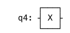
We will use diagrams to represent quantum circuits. Qubits are represented by straight, horizonal lines and gates are represented by boxes on the lines. We can show a single qubit being acted on by a NOT gate as:
acted on by a Z gate as:
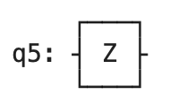
and acted on by a Hadamard gate as:
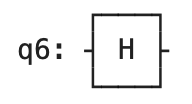
An “M gate” represented the qubit being measured, so the following circuit shows a single qubit being measured:

And the following circuit shows a single qubit being acted on by a Hadamard gate and then measured:
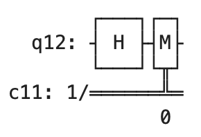
The following are the qiskit imports that are needed to run the remaining code in the notebook. The first import gives you access to the code which is needed to create the quantum circuit, the second import allows you to run your quantum circuit on a simulated quantum computer, and the last piece of code let’s you visualize the results of your simulated quantum computer
# Needed to set up the quantum circuit
from qiskit import QuantumCircuit, ClassicalRegister, QuantumRegister
# Needed to simulate running a quantum computer
from qiskit_aer import AerSimulator
# Neded to visualize the results of running a quantum computer
from qiskit.visualization import plot_histogramThe following code creates a single qubit which is mapped to a single classical qubit for measuring (note this is not always the case and we will discuss why later in the course). The quantum circuit is created, measured, and then drawn.
# creates a Quantum register of 1 qubit
q = QuantumRegister(1)
# creates a classical register of 1 bit
c = ClassicalRegister(1)
# creates a quantum circuit that maps the result of a qubit
# to a classical bit
qc = QuantumCircuit(q, c)
# measure the current quantum circuit and draw a diagram
qc.measure(q, c)
print(qc.draw())
┌─┐
q13: ┤M├
└╥┘
c12: 1/═╩═
0 Now that we have created our quantum circuit we want to run it on a quantum computer. For the majority of this class we will use a simulated quantum computer. The first line of code below creates a simulated quantum computer, the second line of code runs our quantum circuit on the simulated quantum computer and gets the results which are then converted to a histogram with the last line of code.
# Run the quantum circuit on a simulated quantum computer 1024 times
simulator = AerSimulator()
results = simulator.run(qc).result().get_counts()
# Create a histogram of the results
plot_histogram(results)
All Qiskit qubits start in the \(|\uparrow\rangle\) (0) state. This will cause a slight bias to the \(|\uparrow\rangle\) state lateer when we apply gates such as the Hadamard gate.
The below code is similar to what we have already done, but a NOT gate is added to the circuit prior to measuring the state of the circuit. Note that this changes the circuit diagram (with there being both a NOT gate and a measurement “gate” in the circuit diagram) and it changes the results of simulation from all \(|\uparrow\rangle\) (0) to all \(|\downarrow\rangle\) (1) states.
# Create the same quantum circuit as before, but add a NOT gate before
# measuring
q = QuantumRegister(1)
c = ClassicalRegister(1)
qc = QuantumCircuit(q, c)
qc.x(0)
qc.measure(q, c)
print(qc.draw())
simulator = AerSimulator()
results = simulator.run(qc).result().get_counts()
plot_histogram(results)
┌───┐┌─┐
q14: ┤ X ├┤M├
└───┘└╥┘
c13: 1/══════╩═
0 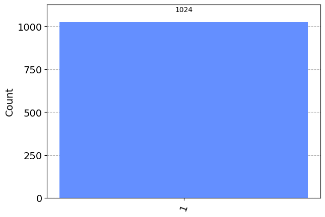
In the below code we have changed the NOT gate to a Z gate, meaning that all of our results have switched back to \(|\uparrow\rangle\) (0) since the Z gate does not change the state of a \(|\uparrow\rangle\) state.
# Replace the NOT gate with a Z gate
q = QuantumRegister(1)
c = ClassicalRegister(1)
qc = QuantumCircuit(q, c)
qc.z(0)
qc.measure(q, c)
print(qc.draw())
simulator = AerSimulator()
results = simulator.run(qc).result().get_counts()
plot_histogram(results)
┌───┐┌─┐
q16: ┤ Z ├┤M├
└───┘└╥┘
c15: 1/══════╩═
0 
Finally, we will replace the Z gate with a Hadamard gate. Note that this is the first example we have of the quantum circuit returning two different results. The results should change every time you run the below cell but the results should remain split roughly equally.
# Replace the Z gate with a Hadamard gate
q = QuantumRegister(1)
c = ClassicalRegister(1)
qc = QuantumCircuit(q, c)
qc.h(0)
qc.measure(q, c)
print(qc.draw())
simulator = AerSimulator()
results = simulator.run(qc).result().get_counts()
plot_histogram(results)
┌───┐┌─┐
q17: ┤ H ├┤M├
└───┘└╥┘
c16: 1/══════╩═
0 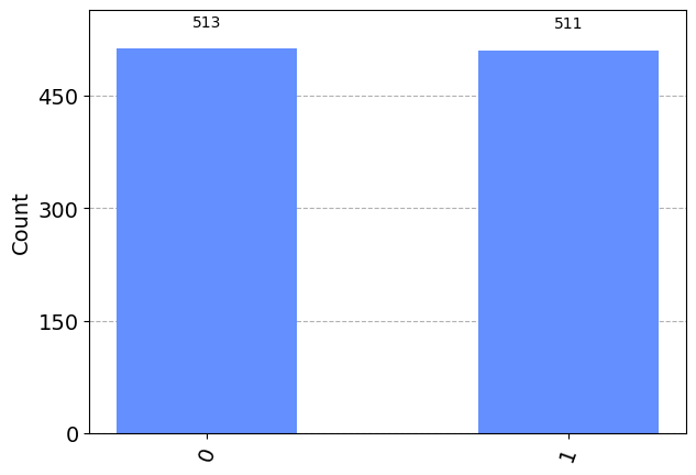
Note that we have applied the Hadamard gate to \(|\uparrow\rangle\) state (since we did not alter the qubit prior to the Hadamard gate) so we have created the \(|+\rangle\) state. This tells us why the simulation results are split roughly 50-50 among the \(|\uparrow\rangle\) and \(|\downarrow\rangle\) states. Since the equation for the \(|+\rangle\) state is \(|+\rangle = \frac{1}{\sqrt{2}}(|\uparrow\rangle + |\downarrow\rangle)\) the probability of measurng \(|+\rangle\) and getting \(|\uparrow\rangle\) is \(|\frac{1}{\sqrt{2}}|^2 = \frac{1}{2}\) (and the same for the \(|\downarrow\rangle\) state since they have the same cofficient).
Based on our discussions above, we can create the \(|-\rangle\) state by applying the Hadamard gate to the \(|\downarrow\rangle\) (1) state. Thus, before the Hadamard gate is applied we need to construct a \(|\downarrow\) state. Since all of the qubits start in the \(|\uparrow\rangle\) state, a simple NOT gate before the Hadamard gate should give us the \(|\downarrow\rangle\) state.
# Replace the Z gate with a Hadamard gate
q = QuantumRegister(1)
c = ClassicalRegister(1)
qc = QuantumCircuit(q, c)
qc.x(0)
qc.h(0)
qc.measure(q, c)
print(qc.draw())
simulator = AerSimulator()
results = simulator.run(qc).result().get_counts()
plot_histogram(results)
┌───┐┌───┐┌─┐
q18: ┤ X ├┤ H ├┤M├
└───┘└───┘└╥┘
c17: 1/═══════════╩═
0 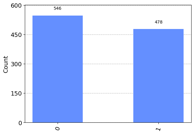
We will use a real quantum computer later in the semester to run our quantum circuits, but there are a couple problems with using a quantum computer initially. The first problem is time. IBM has four quantum computers that it will allows Qiskit users to utilize for free. However, those are shared among every Qiskit user across the world. Thus, when you submit your code to run on a real quantum computer you are placed in a queue and have to wait until the time and space becomes avaliable. Wait times can be quite long (upwards of a day at times) so it slows progress, even when using small circuits.
The second problem os using real quantum computers is quantum noise. Do to a variety of factors (outside interference, trouble maintaining supercool temperatures, etc.) qubits can flip into an undesired state or, when dealing with multiple qubits, become unentangled and no longer work together to solve the problem at hand. To get an idea of how bad this noise can be, the below histogram results from a code creates a single qubit and runs it on a simulated quantum computer with realistic noise (that is with similar errors that you would expect to find on a real quantum computer). Remember that with no gates applied, the qubit should always remain in the \(|\uparrow\rangle\) state. Even though we expect all states to be \(|\uparrow\rangle\) (0), a non-neglible amount of them are in the \(|\downarrow\rangle\) (1) state.
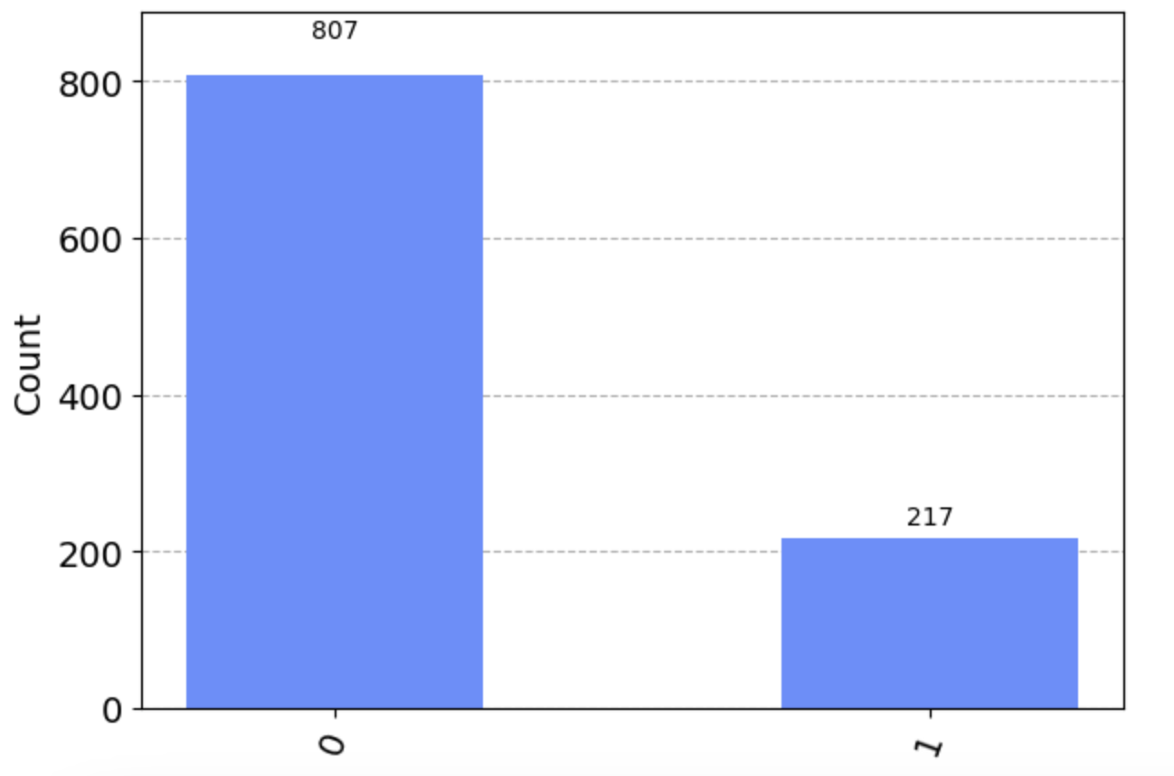
Later in the semester we will learn to deal with quantum noise, but whiel we are initially learning we will use a noiseless simulation both for speed and to ensure that the qubits are in the expected states.
The below code creates a quantum coin flipper which has a theoretical probability of being heads 50% of the time and tails the other 50% of the time.
# creates a Quantum register of 1 qubit
q = QuantumRegister(1)
# creates a classical register of 1 bit
c = ClassicalRegister(1)
# creates a quantum circuit that maps the result of a qubit
# to a classical bit
qc = QuantumCircuit(q, c)
# Apply a Hadamard gate
qc.h(0)
# measure the current quantum circuit and draw a diagram
qc.measure(q, c)
simulator = AerSimulator()
# Only simulate the qubit one time
results = simulator.run(qc, shots=1).result().get_counts()

# There will be only one entry in the results dictionary so see if
# it is a 0. If it is then the result is heads, otherwise its tails
if '0' in results.keys():
    print("Heads!")
else:
    print("Tails!")
Heads!