Model Optimization and Nonlinear Models

Model Optimization and Nonlinear Models#

CSC/DSC 340 Week 5 Slides

Author: Dr. Julie Butler

Date Created: August 19, 2023

Last Modified: September 18, 2023

Plan for the Week#

Monday

Week 5 Pre-Class Homework and Week 4 In-Class Assignment Due

Lecture: Model Optimization and Nonlinear Models

Office Hours: 1pm - 3pm

Tuesday

Office Hours: 4pm - 6pm

Wednesday

Finish Lecture: Model Optimization and Nonlinear Models

Start Week 5 In-Class Assignment

Week 4 Post-Class Homework Due

Thursday

Office Hours: 12:30 - 2pm

Friday

In-Class Assignment Week 5

Problem Analysis Due Before Class (~1 page)

Part 1: Hyperparameter Tuning#

Why do we need hyperparameter tuning?#

The values of the hyperparameters change the output of the model
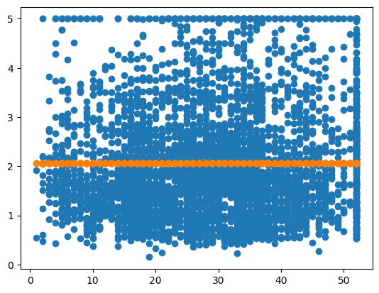
Bad hyperparameters lead to bad results

##############################
##         IMPORTS          ##
##############################
import numpy as np
import matplotlib.pyplot as plt
from sklearn.linear_model import Lasso, Ridge
from sklearn.preprocessing import StandardScaler
from sklearn.model_selection import train_test_split
from sklearn.metrics import mean_squared_error as MSE
from sklearn.datasets import fetch_california_housing

New data set: California Housing
- Goal: Predict the price a house will sale for (house price/100k) given information about the house
- In-Class Week 5

# Print the features
fetch_california_housing().feature_names

['MedInc',
 'HouseAge',
 'AveRooms',
 'AveBedrms',
 'Population',
 'AveOccup',
 'Latitude',
 'Longitude']

##############################
##        IMPORT DATA       ##
##############################
X, y = fetch_california_housing(return_X_y = True)

##############################
##        SCALE DATA        ##
##############################
scaler = StandardScaler()
scaler.fit(X)
Z = scaler.transform(X)

##############################
##     TRAIN-TEST SPLIT     ##
##############################
X_train, X_test, y_train, y_test = train_test_split(Z,y,test_size=0.2)

##############################
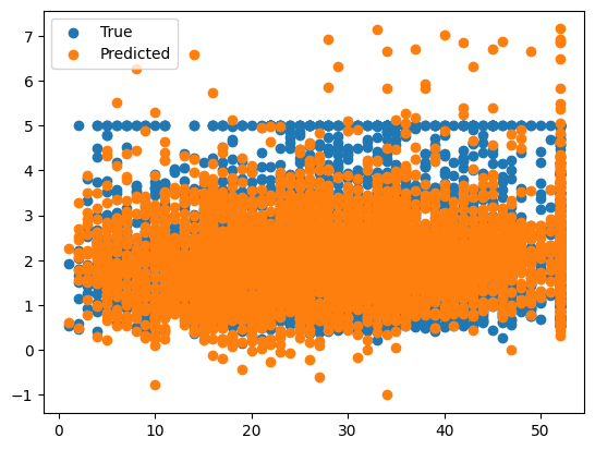
##        GOOD ALPHA        ##
##############################
ridge = Ridge(alpha=1e-15)
ridge.fit(X_train, y_train)
y_pred = ridge.predict(X_test)

err = MSE(y_pred, y_test)
print("MSE:", err)

X_test_plot = scaler.inverse_transform(X_test)

plt.scatter(X_test_plot[:,1],y_test,label='True')
plt.scatter(X_test_plot[:,1],y_pred,label='Predicted')
plt.legend()

MSE: 0.5207853811806975

<matplotlib.legend.Legend at 0x1379a6610>

_images/6f9785647fcb248cb3d3a75e4013899c9306fc6decb84d67692a3b1c60f4cbb3.png

##############################
##        BAD ALPHA         ##
##############################
ridge = Ridge(alpha=1e15)
ridge.fit(X_train, y_train)
y_pred = ridge.predict(X_test)

err = MSE(y_pred, y_test)
print("MSE:", err)

X_test_plot = scaler.inverse_transform(X_test)

plt.scatter(X_test_plot[:,1],y_test,label='True')
plt.scatter(X_test_plot[:,1],y_pred,label='Predicted')

MSE: 1.3166823615106975

<matplotlib.collections.PathCollection at 0x137a58970>

_images/38e5af99f37ca760f52884e701995a5671fa2cb216261a179e44a79471314ff2.png

Methods for Hyperparameter Tuning#

Using Default Values#

Scikit-Learn sets the default value of \(\alpha\) for ridge regression to 1.0, which is a reasonable high level of regularization

# Make the data set smaller (20k+ points in total)
# More points = more data to generate patterns BUT more run time
X = X[:1000]
y = y[:1000]

X_train, X_test, y_train, y_test = train_test_split(X,y,test_size=0.2)

%%time
ridge = Ridge()
ridge.fit(X_train, y_train)
y_pred = ridge.predict(X_test)

CPU times: user 2.43 ms, sys: 5.11 ms, total: 7.54 ms
Wall time: 1.29 ms

err = MSE(y_pred, y_test)
print("MSE:", err)

X_test_plot = scaler.inverse_transform(X_test)

plt.scatter(X_test_plot[:,1],y_test,label='True')
plt.scatter(X_test_plot[:,1],y_pred,label='Predicted')

MSE: 0.3596000507155571

<matplotlib.collections.PathCollection at 0x137b13cd0>

_images/f9f1ea452d2237217e2fecd35f0c464e857043af9c9f6979204d061205fadd6c.png

Pros#

Fast and no need to modify the algorithm

Cons#

Default value may not be the best value, but no test are done to check

For Loop Tuning#

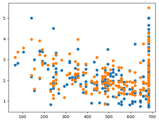
Use a for loop to check many different values for the hyperparameters
Can use nested for loops if more than one hyperparamter

%%time
best_err = 1e4
best_alpha = None
for alpha in np.logspace(-15,4,1000):
    ridge = Ridge(alpha=alpha)
    ridge.fit(X_train, y_train)
    y_pred = ridge.predict(X_test)
    
    err = MSE(y_pred, y_test)
    
    if err < best_err:
        best_err = err
        best_alpha = alpha

CPU times: user 630 ms, sys: 5.05 ms, total: 635 ms
Wall time: 297 ms

ridge = Ridge(alpha=best_alpha)
ridge.fit(X_train, y_train)
y_pred = ridge.predict(X_test)

err = MSE(y_pred, y_test)
print("MSE:", err)
print("CHOSEN ALPHA:", best_alpha)

X_test_plot = scaler.inverse_transform(X_test)

plt.scatter(X_test_plot[:,1],y_test,label='True')
plt.scatter(X_test_plot[:,1],y_pred,label='Predicted')

MSE: 0.3552471269777846
CHOSEN ALPHA: 6.022541201461928e-15

<matplotlib.collections.PathCollection at 0x1076fbb50>

_images/d28f35ca9e6e0b5a29505cd3f63d39728c550f7cf2db13ca034d7948cdf6ad60.png

Pros#

Checks more than one value to find the best value
Simple concept
Short(ish) run times

Cons#

Long piece of code
Not checking all possible values of the hyperparameters

GridSearchCV (Scikit-Learn)#

Scikit-Learn has several hyperparameter tuning implementation
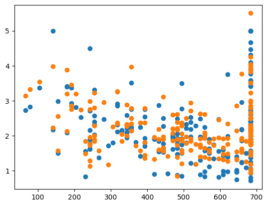
Grid search is a brute force algorithm which checks as many values as given
- If more than one hyperparameter, it checks every single possible combination
“Same” test as for loops but gives much more information, but also takes longer

%%time
from sklearn.model_selection import GridSearchCV

parameters = {'alpha':np.logspace(-15,4,5000)}

ridge = Ridge()

grid_search = GridSearchCV(ridge, parameters,\
                           scoring='neg_mean_squared_error')
grid_search.fit(X_train, y_train)

print(grid_search.best_params_)

{'alpha': 0.20590302760544998}
CPU times: user 13.2 s, sys: 212 ms, total: 13.4 s
Wall time: 13.1 s

ridge = Ridge(alpha=grid_search.best_params_['alpha'])
ridge.fit(X_train, y_train)
y_pred = ridge.predict(X_test)

err = MSE(y_pred, y_test)
print("MSE:", err)
print('CHOSEN ALPHA:', grid_search.best_params_['alpha'])

X_test_plot = scaler.inverse_transform(X_test)

plt.scatter(X_test_plot[:,1],y_test,label='True')
plt.scatter(X_test_plot[:,1],y_pred,label='Predicted')

MSE: 0.3562628152996591
CHOSEN ALPHA: 0.20590302760544998

<matplotlib.collections.PathCollection at 0x137e80a90>

_images/be3d7c2020132424c9c0fc75a9c3df4285aee2ff244fae26985eae19098509d0.png

Pros#

Only takes a few lines to implement
Gives a lot of data once it is fit

Cons#

Long run times
Only searches the range of parameters given

RandomizedSearchCV (Scikit-Learn)#

Tries n_iter randomly chosen values for the hyperparmeters taken from a given distribution (uniform in this case)

%%time
from sklearn.model_selection import RandomizedSearchCV
from scipy.stats import uniform

distributions = {'alpha':uniform(loc=0, scale=4)}

ridge = Ridge()

random_search = RandomizedSearchCV(ridge, distributions,\
                                   scoring='neg_mean_squared_error', n_iter=5000)
random_search.fit(X_train, y_train)

print(random_search.best_params_, random_search.best_score_)

{'alpha': 0.20597888239758078} -0.28856463563603973
CPU times: user 13.3 s, sys: 230 ms, total: 13.5 s
Wall time: 13.2 s

ridge = Ridge(alpha=random_search.best_params_['alpha'])
ridge.fit(X_train, y_train)
y_pred = ridge.predict(X_test)

err = MSE(y_pred, y_test)
print("MSE:", err)
print('CHOSEN ALPHA:', random_search.best_params_['alpha'])

X_test_plot = scaler.inverse_transform(X_test)

plt.scatter(X_test_plot[:,1],y_test,label='True')
plt.scatter(X_test_plot[:,1],y_pred,label='Predicted')

MSE: 0.35626318516764216
CHOSEN ALPHA: 0.20597888239758078

<matplotlib.collections.PathCollection at 0x164bb3940>

Pros#

Only takes a few lines to implement
Gives a lot of data once it is fit

Cons#

Long run times (depending on value of n_iter)
Only searches a finite number of parameter combinations

Bayesian Ridge Regression#

Finds the “most likely” value for \(\alpha\) using Bayesian stastics
Leaves no uncertainity that the best value was just not sampled

%%time
from sklearn.linear_model import BayesianRidge

bayesian_ridge = BayesianRidge()
bayesian_ridge.fit(X_train, y_train)
y_pred = bayesian_ridge.predict(X_test)

print(bayesian_ridge.alpha_)

3.688440522864384
CPU times: user 5.58 ms, sys: 1.28 ms, total: 6.85 ms
Wall time: 1.68 ms

ridge = BayesianRidge()
ridge.fit(X_train, y_train)
y_pred = ridge.predict(X_test)

err = MSE(y_pred, y_test)
print("MSE:", err)
print('CHOSEN ALPHA:', ridge.alpha_)

X_test_plot = scaler.inverse_transform(X_test)

plt.scatter(X_test_plot[:,1],y_test,label='True')
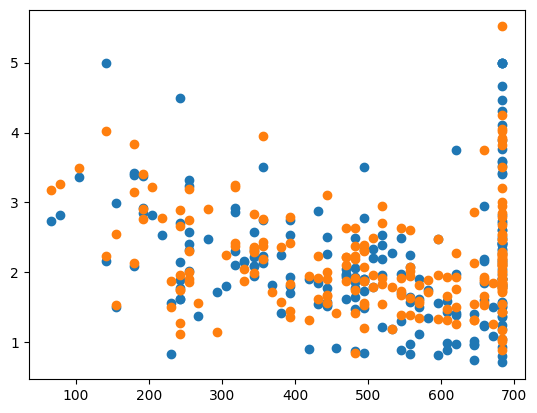
plt.scatter(X_test_plot[:,1],y_pred,label='Predicted')

MSE: 0.3592175812997633
CHOSEN ALPHA: 3.688440522864384

<matplotlib.collections.PathCollection at 0x164d18610>

_images/e54df8ad8187114ee8728134157bd7bea58fc69dec202cd228fb60f1dfa7622b.png

Pros#

Only takes a few lines to implement
Statical certainity that the given \(\alpha\) value is the best value
Short run times

Cons#

Only valid for Bayesian ridge regression (linear model)

Comparison of \(\alpha\), Accuracy, and Run Time#

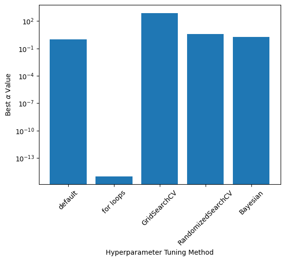
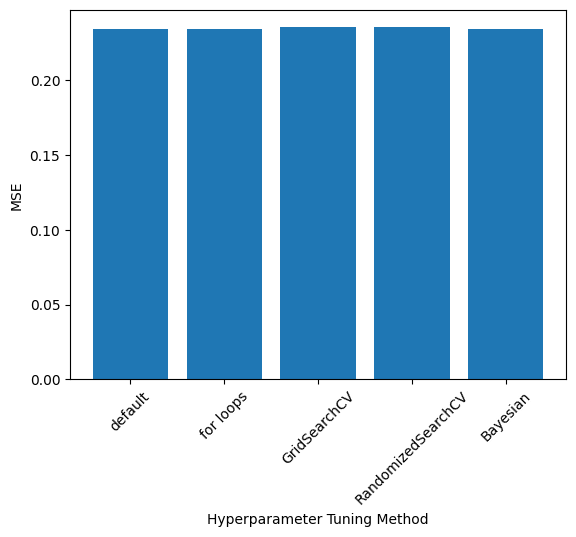
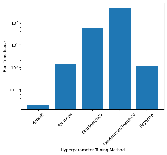
Exact values depend on the train-test split and RandomizedSearch results; these values were taken from one run

labels = ['default', 'for loops', 'GridSearchCV', 'RandomizedSearchCV', 'Bayesian']
alphas = [1.0, 1e-15, 769.79, 3.99, 1.90]
mse = [0.23461613368850237, 0.2343672966024232, 0.23546465060931623, 0.23546192678932165, 0.23439940455100014]
run_times = [20.8/1000, 1.35, 57.7, 7*60+40, 1.18] #ms

plt.bar(np.arange(0,len(labels)), alphas)
plt.yscale('log')
plt.xticks(np.arange(0,len(labels)), labels, rotation=45)
plt.ylabel(r"Best $\alpha$ Value")
plt.xlabel("Hyperparameter Tuning Method")

Text(0.5, 0, 'Hyperparameter Tuning Method')

_images/6a146f227e2ade44e574e781891a2688e2a1d6a13a4aa04842c1e01cce9d4935.png

plt.bar(np.arange(0,len(labels)), mse)
plt.xticks(np.arange(0,len(labels)), labels, rotation=45)
plt.ylabel(r"MSE")
plt.xlabel("Hyperparameter Tuning Method")

Text(0.5, 0, 'Hyperparameter Tuning Method')

_images/c569609b03b2b8cd2958ff13526a5371972b26bb99fe955c13411ce0675694cf.png

plt.bar(np.arange(0,len(labels)), run_times)
plt.xticks(np.arange(0,len(labels)), labels, rotation=45)
plt.ylabel(r"Run Time (sec.)")
plt.xlabel("Hyperparameter Tuning Method")
plt.yscale('log')

_images/6ffca5b6552a25ce1daeee7c6dd051b600e5366e43c192552a1ac3f360b41b54.png

Part 2: Feature Engineering#

Feature engineering is the process of eliminating or altering given inputs in order to improve the model’s predictions

Design matrix/alter the inputs
Remove features that are not useful
Scaling the features or targets

import pandas as pd
import seaborn as sns

housing = fetch_california_housing()

housing_data = pd.DataFrame(housing.data, columns=housing.feature_names)

housing_data['target'] = housing.target

housing_data = housing_data.sample(1000)

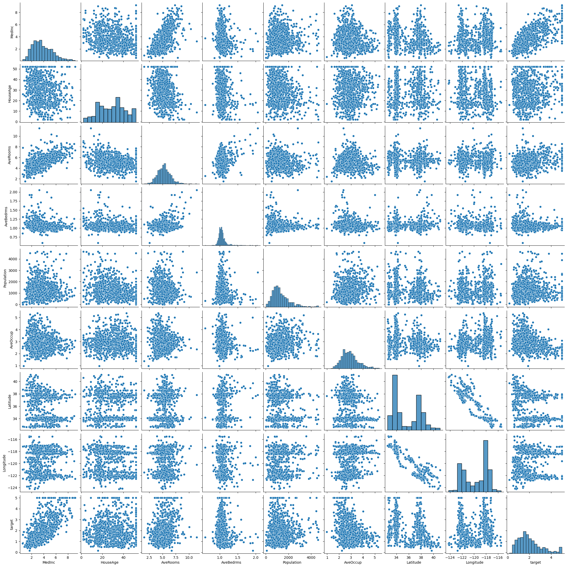
Pairplots can give us initial ideas about the data set and and obvious relations

sns.pairplot(housing_data)

/Users/juliehartley/Library/Python/3.9/lib/python/site-packages/seaborn/axisgrid.py:118: UserWarning: The figure layout has changed to tight
  self._figure.tight_layout(*args, **kwargs)

<seaborn.axisgrid.PairGrid at 0x164247e20>

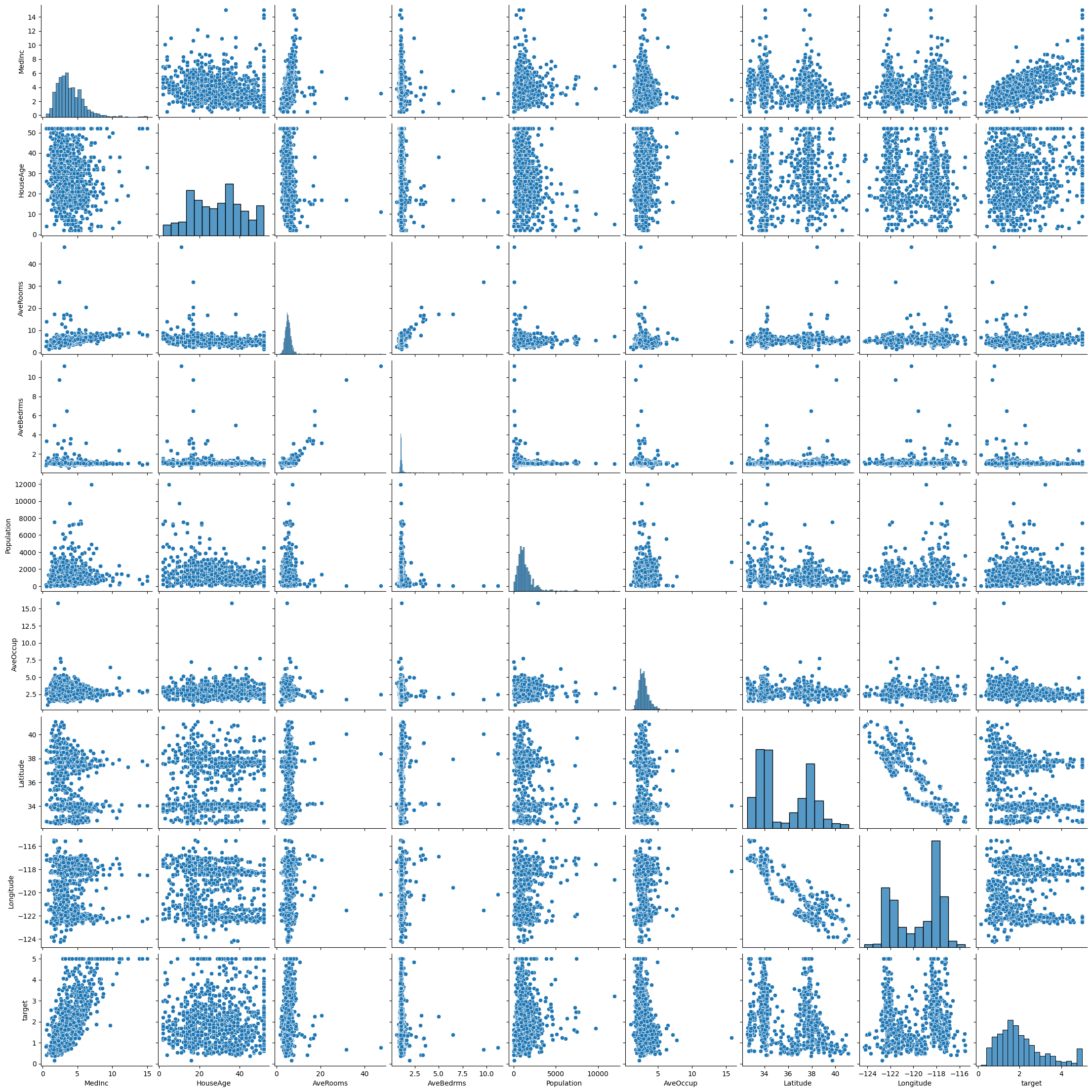
_images/129d47b1868a2f5ad7333f6073ef3d2aa6d8f7b5ec0f42cc4557f3968a164207.png

# Remove outliers from the data set and make the pairplot again

from scipy import stats

housing_data = housing_data[(np.abs(stats.zscore(housing_data)) < 3).all(axis=1)]

sns.pairplot(housing_data)

/Users/juliehartley/Library/Python/3.9/lib/python/site-packages/seaborn/axisgrid.py:118: UserWarning: The figure layout has changed to tight
  self._figure.tight_layout(*args, **kwargs)

<seaborn.axisgrid.PairGrid at 0x1689a4070>

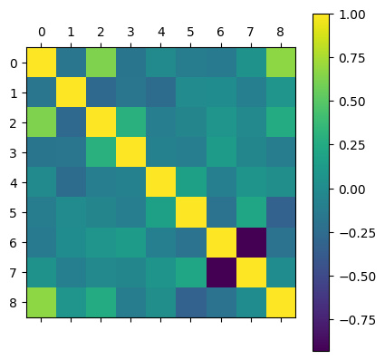
_images/048bfb225ecfd5c6a29aa2c5b26b57f6477702c32bcd6f9e705df8aaeafd5ef8.png

Correlation Matrix#

Correlation score = \(\sqrt{R2\ Score}\)
Values close to \(\pm1\) means that the two feautures are linearly related

correlation_matrix = housing_data.corr()
correlation_matrix

	MedInc	HouseAge	AveRooms	AveBedrms	Population	AveOccup	Latitude	Longitude	target
MedInc	1.000000	-0.176376	0.624278	-0.182821	-0.006504	-0.118286	-0.145364	0.051990	0.671977
HouseAge	-0.176376	1.000000	-0.273970	-0.171407	-0.250648	-0.000109	0.007118	-0.100684	0.077059
AveRooms	0.624278	-0.273970	1.000000	0.292713	-0.108061	-0.049828	0.077900	-0.022613	0.254047
AveBedrms	-0.182821	-0.171407	0.292713	1.000000	-0.080388	-0.102396	0.132675	-0.047917	-0.121542
Population	-0.006504	-0.250648	-0.108061	-0.080388	1.000000	0.170063	-0.097118	0.070431	0.019527
AveOccup	-0.118286	-0.000109	-0.049828	-0.102396	0.170063	1.000000	-0.198600	0.214724	-0.324090
Latitude	-0.145364	0.007118	0.077900	0.132675	-0.097118	-0.198600	1.000000	-0.931286	-0.198935
Longitude	0.051990	-0.100684	-0.022613	-0.047917	0.070431	0.214724	-0.931286	1.000000	0.006876
target	0.671977	0.077059	0.254047	-0.121542	0.019527	-0.324090	-0.198935	0.006876	1.000000

plt.matshow(correlation_matrix)
plt.colorbar()

<matplotlib.colorbar.Colorbar at 0x28b885fd0>

_images/a4820a25a199faef10a309b371527a6d2bbb998debb3e7cbcf3171e12975ca38.png

LASSO Regression for Feature Selection#

lasso = Lasso()
lasso.fit(X,y)
ypred = lasso.predict(X)
print(MSE(ypred,y))
lasso.coef_

0.638471842835069

array([ 0.06161184, -0.        ,  0.        , -0.        ,  0.00011673,
       -0.        ,  0.        ,  0.        ])

Accuracy with All Data (Scaled)#

X = housing_data.drop(columns=['target'])
y = housing_data['target']

scaler = StandardScaler()
scaler.fit(X)
Z = scaler.transform(X)

X_train, X_test, y_train, y_test = train_test_split(Z,y,test_size=0.2)

bayesian_ridge = BayesianRidge()
bayesian_ridge.fit(X_train, y_train)
y_pred = bayesian_ridge.predict(X_test)

print('MSE:', MSE(y_pred, y_test))

MSE: 0.44933334607255193

Accuracy with Most Correlated Features (Scaled)#

X_corr = housing_data[['MedInc', 'HouseAge', 'AveRooms']]
y = housing_data['target']

scaler = StandardScaler()
scaler.fit(X_corr)
Z = scaler.transform(X_corr)

X_train, X_test, y_train, y_test = train_test_split(Z,y,test_size=0.2)

bayesian_ridge = BayesianRidge()
bayesian_ridge.fit(X_train, y_train)
y_pred = bayesian_ridge.predict(X_test)

print('MSE:', MSE(y_pred, y_test))

MSE: 0.5527782905639612

Automate the dimensionality reduction with unsupervised learning (next week!)

Part 3: Nonlinear Models#

Kernel Ridge Regression (KRR)#

All previous models we have studied have been linear–capable of modeling linear patterns
- Design matrices can only add some much functions
Many data sets will have a nonlinear pattern and thus we need a nonlinear model
- Kernel ridge regression (KRR)
- Support vector machines (SVMs)
- Neural Networks

Kernel Functions#

Scikit-Learn kernels are found here
- Linear: \(k(x,y) = x^Ty\)
- Polynomial: k(x,y) = \((\gamma x^Ty+c_0)^d\)
- Sigmoid: \(k(x,y) = tanh(\gamma x^Ty+c_0)\)
- Radial Basis Function (RBF): \(k(x,y) = exp(-\gamma||x-y||_2)\)
Inputs to KRR algorithm are modified by the kernel function, thus giving the method nonlinearuty \(\longrightarrow\) kernel methods/trick allows linear methods to solve nonlinear problems
- Kernel ridge regression is just ridge regression with the inputs modified by the kernel function

KRR Equations#

Form of predictions: \(\hat{y}(x) = \sum_{i=1}^m \theta_ik(x_i,x)\)
Loss function:\(J(\theta) = MSE(y,\hat{y}) + \frac{\alpha}{2}\sum_{i=1}^n\theta_i^2\)
Optimized parameters: \(\theta = (\textbf{K}-\alpha\textbf{I})^{-1}y\)
- \(\textbf{K} = k(x_i, x_j)\)

Hyperparameter Tuning with Many Hyperparameters#

KRR has the same hyperparameter as ridge regression: \(\alpha\)
Each kernel function has 0-3 hyperparameters
The choice of kernel function is a hyperparameter
Hyperparameter tuning becomes more important as the number of hyperparameters in the model increases

Housing Data with Kernel Ridge Regression#

from sklearn.kernel_ridge import KernelRidge

X,y = fetch_california_housing(return_X_y=True)

X = X[:500]
y = y[:500]

scaler = StandardScaler()
scaler.fit(X)
Z = scaler.transform(X)

X_train, X_test, y_train, y_test = train_test_split(Z,y,test_size=0.2)

krr = KernelRidge()
krr.fit(X_train, y_train)
y_pred = krr.predict(X_test)
print("MSE:", MSE(y_pred, y_test))

MSE: 4.105741823609707

distributions = {'alpha':uniform(loc=0, scale=4), 'kernel':['linear', \
                                                            'polynomial', 'rbf', \
                                                            'sigmoid', 'laplacian'], \
                 'gamma':uniform(loc=0, scale=4),\
                'degree':np.arange(0,10), 'coef0':uniform(loc=0, scale=4)}

krr = KernelRidge()

random_search = RandomizedSearchCV(krr, distributions,\
                                   scoring='neg_mean_squared_error', n_iter=50)
random_search.fit(X_train, y_train)
print(random_search)
print(random_search.best_params_, random_search.best_score_)

---------------------------------------------------------------------------
KeyboardInterrupt                         Traceback (most recent call last)
Cell In [32], line 11
krr = KernelRidge()
random_search = RandomizedSearchCV(krr, distributions,\
                                  scoring='neg_mean_squared_error', n_iter=50)
---> 11 random_search.fit(X_train, y_train)
print(random_search)
print(random_search.best_params_, random_search.best_score_)

File ~/Library/Python/3.9/lib/python/site-packages/sklearn/model_selection/_search.py:875, in BaseSearchCV.fit(self, X, y, groups, **fit_params)
   results = self._format_results(
       all_candidate_params, n_splits, all_out, all_more_results
   )
   return results
--> 875 self._run_search(evaluate_candidates)
# multimetric is determined here because in the case of a callable
# self.scoring the return type is only known after calling
first_test_score = all_out[0]["test_scores"]

File ~/Library/Python/3.9/lib/python/site-packages/sklearn/model_selection/_search.py:1753, in RandomizedSearchCV._run_search(self, evaluate_candidates)
def _run_search(self, evaluate_candidates):
   """Search n_iter candidates from param_distributions"""
-> 1753     evaluate_candidates(
       ParameterSampler(
           self.param_distributions, self.n_iter, random_state=self.random_state
       )
   )

File ~/Library/Python/3.9/lib/python/site-packages/sklearn/model_selection/_search.py:822, in BaseSearchCV.fit.<locals>.evaluate_candidates(candidate_params, cv, more_results)
if self.verbose > 0:
   print(
       "Fitting {0} folds for each of {1} candidates,"
       " totalling {2} fits".format(
           n_splits, n_candidates, n_candidates * n_splits
       )
   )
--> 822 out = parallel(
   delayed(_fit_and_score)(
       clone(base_estimator),
       X,
       y,
       train=train,
       test=test,
       parameters=parameters,
       split_progress=(split_idx, n_splits),
       candidate_progress=(cand_idx, n_candidates),
       **fit_and_score_kwargs,
   )
   for (cand_idx, parameters), (split_idx, (train, test)) in product(
       enumerate(candidate_params), enumerate(cv.split(X, y, groups))
   )
)
if len(out) < 1:
   raise ValueError(
       "No fits were performed. "
       "Was the CV iterator empty? "
       "Were there no candidates?"
   )

File ~/Library/Python/3.9/lib/python/site-packages/joblib/parallel.py:1088, in Parallel.__call__(self, iterable)
if self.dispatch_one_batch(iterator):
   self._iterating = self._original_iterator is not None
-> 1088 while self.dispatch_one_batch(iterator):
   pass
if pre_dispatch == "all" or n_jobs == 1:
   # The iterable was consumed all at once by the above for loop.
   # No need to wait for async callbacks to trigger to
   # consumption.

File ~/Library/Python/3.9/lib/python/site-packages/joblib/parallel.py:901, in Parallel.dispatch_one_batch(self, iterator)
   return False
else:
--> 901     self._dispatch(tasks)
   return True

File ~/Library/Python/3.9/lib/python/site-packages/joblib/parallel.py:819, in Parallel._dispatch(self, batch)
with self._lock:
   job_idx = len(self._jobs)
--> 819     job = self._backend.apply_async(batch, callback=cb)
   # A job can complete so quickly than its callback is
   # called before we get here, causing self._jobs to
   # grow. To ensure correct results ordering, .insert is
   # used (rather than .append) in the following line
   self._jobs.insert(job_idx, job)

File ~/Library/Python/3.9/lib/python/site-packages/joblib/_parallel_backends.py:208, in SequentialBackend.apply_async(self, func, callback)
def apply_async(self, func, callback=None):
   """Schedule a func to be run"""
--> 208     result = ImmediateResult(func)
   if callback:
       callback(result)

File ~/Library/Python/3.9/lib/python/site-packages/joblib/_parallel_backends.py:597, in ImmediateResult.__init__(self, batch)
def __init__(self, batch):
   # Don't delay the application, to avoid keeping the input
   # arguments in memory
--> 597     self.results = batch()

File ~/Library/Python/3.9/lib/python/site-packages/joblib/parallel.py:288, in BatchedCalls.__call__(self)
def __call__(self):
   # Set the default nested backend to self._backend but do not set the
   # change the default number of processes to -1
   with parallel_backend(self._backend, n_jobs=self._n_jobs):
--> 288         return [func(*args, **kwargs)
               for func, args, kwargs in self.items]

File ~/Library/Python/3.9/lib/python/site-packages/joblib/parallel.py:288, in <listcomp>(.0)
def __call__(self):
   # Set the default nested backend to self._backend but do not set the
   # change the default number of processes to -1
   with parallel_backend(self._backend, n_jobs=self._n_jobs):
--> 288         return [func(*args, **kwargs)
               for func, args, kwargs in self.items]

File ~/Library/Python/3.9/lib/python/site-packages/sklearn/utils/fixes.py:117, in _FuncWrapper.__call__(self, *args, **kwargs)
def __call__(self, *args, **kwargs):
   with config_context(**self.config):
--> 117         return self.function(*args, **kwargs)

File ~/Library/Python/3.9/lib/python/site-packages/sklearn/model_selection/_validation.py:686, in _fit_and_score(estimator, X, y, scorer, train, test, verbose, parameters, fit_params, return_train_score, return_parameters, return_n_test_samples, return_times, return_estimator, split_progress, candidate_progress, error_score)
       estimator.fit(X_train, **fit_params)
   else:
--> 686         estimator.fit(X_train, y_train, **fit_params)
except Exception:
   # Note fit time as time until error
   fit_time = time.time() - start_time

File ~/Library/Python/3.9/lib/python/site-packages/sklearn/kernel_ridge.py:195, in KernelRidge.fit(self, X, y, sample_weight)
   ravel = True
copy = self.kernel == "precomputed"
--> 195 self.dual_coef_ = _solve_cholesky_kernel(K, y, alpha, sample_weight, copy)
if ravel:
   self.dual_coef_ = self.dual_coef_.ravel()

File ~/Library/Python/3.9/lib/python/site-packages/sklearn/linear_model/_ridge.py:249, in _solve_cholesky_kernel(K, y, alpha, sample_weight, copy)
K.flat[:: n_samples + 1] += alpha[0]
try:
   # Note: we must use overwrite_a=False in order to be able to
   #       use the fall-back solution below in case a LinAlgError
   #       is raised
--> 249     dual_coef = linalg.solve(K, y, assume_a="pos", overwrite_a=False)
except np.linalg.LinAlgError:
   warnings.warn(
       "Singular matrix in solving dual problem. Using "
       "least-squares solution instead."
   )

File ~/Library/Python/3.9/lib/python/site-packages/scipy/linalg/_basic.py:251, in solve(a, b, lower, overwrite_a, overwrite_b, check_finite, assume_a, transposed)
# Positive definite case 'posv'
else:
   pocon, posv = get_lapack_funcs(('pocon', 'posv'),
                                  (a1, b1))
--> 251     lu, x, info = posv(a1, b1, lower=lower,
                      overwrite_a=overwrite_a,
                      overwrite_b=overwrite_b)
   _solve_check(n, info)
   rcond, info = pocon(lu, anorm)

KeyboardInterrupt: 

X,y = fetch_california_housing(return_X_y=True)

scaler = StandardScaler()
scaler.fit(X)
Z = scaler.transform(X)

X_train, X_test, y_train, y_test = train_test_split(Z,y,test_size=0.2)

# Using the best parameters from through one run of the 
# RandomizedSearchCV method above
krr = KernelRidge(alpha= 0.35753693232459094, coef0= 3.2725118241858264, degree= 9, gamma= 0.14696609545731532, kernel= 'laplacian')
krr.fit(X_train, y_train)
y_pred = krr.predict(X_test)
print('MSE:', MSE(y_pred, y_test))

MSE: 0.23499324697787755

bayesian_ridge = BayesianRidge()
bayesian_ridge.fit(X_train, y_train)
y_pred = bayesian_ridge.predict(X_test)
print('MSE:', MSE(y_pred, y_test))

MSE: 0.5242651488478602

Model Optimization and Nonlinear Models

Contents

Model Optimization and Nonlinear Models#

Plan for the Week#

Part 1: Hyperparameter Tuning#

Why do we need hyperparameter tuning?#

Methods for Hyperparameter Tuning#

Using Default Values#

Pros#

Cons#

For Loop Tuning#

Pros#

Cons#

GridSearchCV (Scikit-Learn)#

Pros#

Cons#

RandomizedSearchCV (Scikit-Learn)#

Pros#

Cons#

Bayesian Ridge Regression#

Pros#

Cons#

Comparison of \(\alpha\), Accuracy, and Run Time#

Part 2: Feature Engineering#

Correlation Matrix#

LASSO Regression for Feature Selection#

Accuracy with All Data (Scaled)#

Accuracy with Most Correlated Features (Scaled)#

Part 3: Nonlinear Models#

Kernel Ridge Regression (KRR)#

Kernel Functions#

KRR Equations#

Hyperparameter Tuning with Many Hyperparameters#

Housing Data with Kernel Ridge Regression#