Creating Neural Networks from Scratch#
CSC/DSC 340 Week 9 Slides
Author: Dr. Julie Butler
Date Created: October 16, 2023
Last Modified: October 16, 2023
This week we will learn how to create neural networks from scratch, using the Python library JAX to perform the optimization.
Another common library for this task is autograd but it is no longer being maintained
Review of Neural Network Equations#
A return to Week 7 Slides
Creating a Neural Network from Scratch Using JAX#
JAX is an automatic differentiation library in Python that can find the derivative of any chunk of code it is given.
If you are interested you can read more about the library here.
# IMPORTS
# Math for the ceiling function
from math import ceil
# Matplotlib for graphing capabilities
from matplotlib import pyplot as plt
# Numpy for arrays
import numpy as np
# Modules from the JAX library for creating neural networks
import jax.numpy as jnp
from jax import grad
from jax import random as npr
Generate the Data Set#
Let’s keep things simple and generate a data points from a Gaussian curve. We will have our x data be evenly space between -10 and 10 and our y data be the corresponding points on a Gaussian curve.
# Let's create a data set that is just a basic Gaussian curve
X = np.linspace(-10,10,250)
y = np.exp(-X**2)
Perform a Train-Test Split#
# We will split the data set into two pieces, a training data set that contains
# 80% of the total data and a test set that contains the other 20%
from sklearn.model_selection import train_test_split
train_size = 0.8
X_train, X_test, y_train, y_test = train_test_split(X, y, train_size=train_size)
Define the Neural Network#
First we will define the sigmoid function as our activation function.
def sigmoid(x):
    """
        Calculates the value of the sigmoid function for
        a given input of x
    """
    return 1. / (1. + jnp.exp(-x))
Now we will define our neural network.
Here we will be using an architecture with two hidden layers, each using the sigmoid activation function, and an output layer which does not have an activation function.
Note that we do not use the bias offset in this code
def neural_network(W, x):
    """
        Inputs:
            W (a list): the weights of the neural network
            x (a float): the input value of the neural network
        Returns:
            Unnamed (a float): The output of the neural network
        Defines a neural network with one hidden layer.  The number of neurons in
        the hidden layer is the length of W[0]. The activation function is the
        sigmoid function on the hidden layer an none on the output layer.
    """
    # Calculate the output for the neurons in the hidden layers
    hidden_layer1 = sigmoid(jnp.dot(x,W[0]))
    hidden_layer2 = sigmoid(jnp.dot(hidden_layer1, W[1]))
    # Calculate the result for the output neuron
    return jnp.dot(hidden_layer2, W[2])
Define the Loss Function#
Now we need to define our loss function. For simplicity we will be using the mean-squared error loss function, which is a very common loss function for training neural networks.
def loss_function(W, x, y):
    """
        Inputs:
            W (a list): the weights of the neural network
            t (a 1D NumPy array): the times to calculate the predicted position at
        Returns:
            loss_sum (a float): The total loss over all times
        The loss function for the neural network to solve for position given
        a function for acceleration.
    """
    # Define a variable to hold the total loss
    loss_sum = 0.
    # Loop through each individual time
    for i in range(len(x)):
        # Get the output of the neural network with the given set of weights
        nn = neural_network(W, x[i])[0][0]
        err_sqr = (nn-y[i])**2
        # Update the loss sum
        loss_sum += err_sqr
    loss_sum /= len(x)
    # Return the loss sum
    return loss_sum
Train the Neural Network#
Finally we need to train our neural network.
We will start by randomly initializing the weights of our neural network (with 25 neurons per hidden layer).
# Generate the key for the random number generator
key = npr.PRNGKey(0)
# Set the number of neurons in the hidden layer
number_hidden_neurons = 25
# Initialize the weights of the neural network with random numbers
W = [npr.normal(key,(1, number_hidden_neurons)),
     npr.normal(key,(number_hidden_neurons,number_hidden_neurons)),
     npr.normal(key,(number_hidden_neurons, 1))]
We then define the parameters for the learning rate, the number of training iterations, and the threshold for stopping the training.
# Set the learning rate and the number of training iterations for the network
learning_rate = 0.01
num_training_iterations = 100
threshold = 0.0001
previous_loss = 0
Next, we perform gradient descent to update the weights of the neural network over for the set number of training iterations, or until the loss function value converges to some set threshold.
WARNING: This cell will take a long time to run.
# Train the neural network for the specified number of iterations
# Update the weights using the learning rates
for i in range(num_training_iterations):
    print("Training Iteration:", i+1)
    current_loss = loss_function(W,X_train,y_train)
    print("Loss:", current_loss)
    print()
    # If the current loss is within a set threshold of the previous loss, stop
    # the training
    if np.abs(current_loss-previous_loss) < threshold:
        break;
    # Calculate the gradient of the loss function and then use that gradient to
    # update the weights of the neural network using the learning rate and the
    # gradient descent optimization method
    loss_grad =  grad(loss_function)(W, X_train, y_train)
    # Update first hidden layer
    W[0] = W[0] - learning_rate * loss_grad[0]
    # Update second hidden layer
    W[1] = W[1] - learning_rate * loss_grad[1]
    # Update output layer
    W[2] = W[2] - learning_rate * loss_grad[2]
    previous_loss = current_loss
Training Iteration: 1
Loss: 5.3948293
Training Iteration: 2
Loss: 3.73042
Training Iteration: 3
Loss: 2.6401887
Training Iteration: 4
Loss: 1.9165754
Training Iteration: 5
Loss: 1.428656
Training Iteration: 6
Loss: 1.0936975
Training Iteration: 7
Loss: 0.85916555
Training Iteration: 8
Loss: 0.69148195
Training Iteration: 9
Loss: 0.5690006
Training Iteration: 10
Loss: 0.4776287
Training Iteration: 11
Loss: 0.40808192
Training Iteration: 12
Loss: 0.35415912
Training Iteration: 13
Loss: 0.31165215
Training Iteration: 14
Loss: 0.27765605
Training Iteration: 15
Loss: 0.25012755
Training Iteration: 16
Loss: 0.22760028
Training Iteration: 17
Loss: 0.20900093
Training Iteration: 18
Loss: 0.19352901
Training Iteration: 19
Loss: 0.18057571
Training Iteration: 20
Loss: 0.1696702
Training Iteration: 21
Loss: 0.16044348
Training Iteration: 22
Loss: 0.15260157
Analyze the Results#
Now we need to analyze the performance of our neural network using the test data set that was reserved earlier. First we need to generate the neural network predictions for the y component of the test data set.
y_nn = [neural_network(W, xi)[0][0] for xi in X_test]
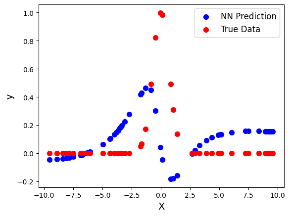
First lets analyze the results graphically by plotting the predicted test data set and the true test data set on the same graph.
plt.scatter(X_test, y_nn, s=50, color="blue",label="NN Prediction")
plt.scatter(X_test, y_test, s=50, color="red", label="True Data")
plt.legend(fontsize=12)
plt.xlabel("X",fontsize=14)
plt.ylabel("y",fontsize=14)
Text(0, 0.5, 'y')

Next let’s analyze the error numerically using the root mean-squared error (RMSE) function, which is simiply the square root of the mean-squared error. The RMSE gives the average error on each data point (instead of the squared average error) so it is a met more of a clear metric for error analysis. First, let’s define a function to calculate the RMSE between two data sets.
def rmse(A,B):
    """
        Inputs:
            A,B (NumPy arrays)
        Returns:
            Unnamed (a float): the RMSE error between A and B
        Calculates the RMSE error between A and B.
    """
    assert len(A)==len(B),"The data sets must be the same length to calcualte\
        the RMSE."
    return np.sqrt(np.average((A-B)**2))
Now let’s print the RMSE between the true test data set and the neural network prediction.
print("RMSE between true test set and neural network result:", rmse(y_nn,y_test))
RMSE between true test set and neural network result: 0.28406674843753915

